1. Introduction: How Cylc Works

This section of the user guide is being rewritten for Cylc 8. For the moment we’ve removed some outdated information, leaving just the description of how Cylc manages cycling workflows. For a more up-to-date description see references cited on the Cylc web site.

1.1. Dependence Between Tasks

1.1.1. Intra-cycle Dependence

Most dependence between tasks applies within a single cycle point. Fig. 1 shows the dependency diagram for a single cycle point of a simple example suite of three scientific models (say) (a, b, and c) and three post processing or product generation tasks (d, e and f). A scheduler capable of handling this must manage, within a single cycle point, multiple parallel streams of execution that branch when one task generates output for several downstream tasks, and merge when one task takes input from several upstream tasks.

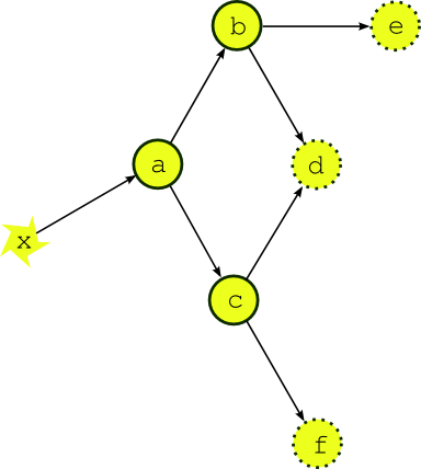
Fig. 1 A single cycle point dependency graph for a simple suite. The dependency graph for a single cycle point of a simple example suite. Tasks a, b, and c represent models, d, e and f are post processing or product generation tasks, and x represents external data that the upstream model depends on.

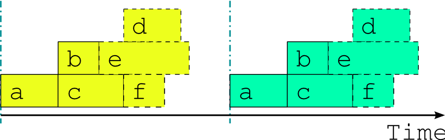
Fig. 2 A single cycle point job schedule for real time operation. The optimal job schedule for two consecutive cycle points of our example suite during real time operation, assuming that all tasks trigger off upstream tasks finishing completely. The horizontal extent of a task bar represents its execution time, and the vertical blue lines show when the external driving data becomes available.

Fig. 2 shows the optimal job schedule for two consecutive cycle points of the example suite in real time operation, given execution times represented by the horizontal extent of the task bars. There is a time gap between cycle points as the suite waits on new external driving data. Each task in the example suite happens to trigger off upstream tasks finishing, rather than off any intermediate output or event; this is merely a simplification that makes for clearer diagrams.

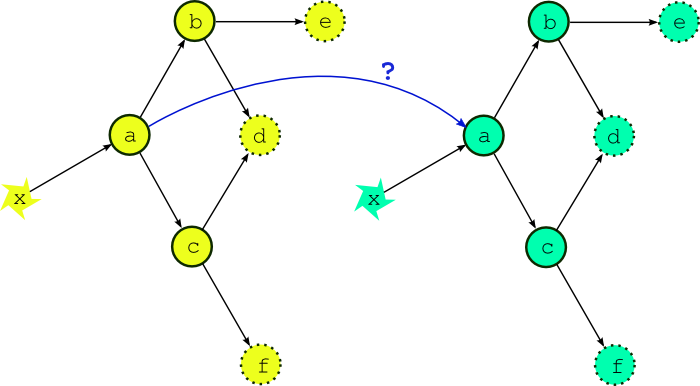
Fig. 3 What if the external driving data is available early? If the external driving data is available in advance, can we start running the next cycle point early?

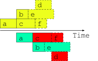
Fig. 4 Attempted overlap of consecutive single-cycle-point job schedules. A naive attempt to overlap two consecutive cycle points using the single-cycle-point dependency graph. The red shaded tasks will fail because of dependency violations (or will not be able to run because of upstream dependency violations).

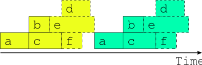
Fig. 5 The only safe multi-cycle-point job schedule? The best that can be done in general when inter-cycle dependence is ignored.

Now the question arises, what happens if the external driving data for upcoming cycle points is available in advance, as it would be after a significant delay in operations, or when running a historical case study? While the model a appears to depend only on the external data x, in fact it could also depend on its own previous instance for the model background state used in initializing the new run (this is almost always the case for atmospheric models used in weather forecasting). Thus, as alluded to in Fig. 3, task a could in principle start as soon as its predecessor has finished. Fig. 4 shows, however, that starting a whole new cycle point at this point is dangerous - it results in dependency violations in half of the tasks in the example suite. In fact the situation could be even worse than this - imagine that task b in the first cycle point is delayed for some reason after the second cycle point has been launched. Clearly we must consider handling inter-cycle dependence explicitly or else agree not to start the next cycle point early, as is illustrated in Fig. 5.

1.1.2. Inter-Cycle Dependence

Wether forecast models typically depend on their own most recent previous forecast for background state or restart files of some kind (this is called warm cycling) but there can also be inter-cycle dependence between other tasks. In an atmospheric forecast analysis suite, for instance, the weather model may generate background states for observation processing and data-assimilation tasks in the next cycle point as well as for the next forecast model run. In real time operation inter-cycle dependence can be ignored because it is automatically satisfied when one cycle point finishes before the next begins. If it is not ignored it drastically complicates the dependency graph by blurring the clean boundary between cycle points. Fig. 6 illustrates the problem for our simple example suite assuming minimal inter-cycle dependence: the warm cycled models (a, b, and c) each depend on their own previous instances.

For this reason, and because we tend to see forecasting suites in terms of their real time characteristics, other metaschedulers have ignored inter-cycle dependence and are thus restricted to running entire cycle points in sequence at all times. This does not affect normal real time operation but it can be a serious impediment when advance availability of external driving data makes it possible, in principle, to run some tasks from upcoming cycle points before the current cycle point is finished - as was suggested at the end of the previous section. This can occur, for instance, after operational delays (late arrival of external data, system maintenance, etc.) and to an even greater extent in historical case studies and parallel test suites started behind a real time operation. It can be a serious problem for suites that have little downtime between forecast cycle points and therefore take many cycle points to catch up after a delay. Without taking account of inter-cycle dependence, the best that can be done, in general, is to reduce the gap between cycle points to zero as shown in Fig. 5. A limited crude overlap of the single cycle point job schedule may be possible for specific task sets but the allowable overlap may change if new tasks are added, and it is still dangerous: it amounts to running different parts of a dependent system as if they were not dependent and as such it cannot be guaranteed that some unforeseen delay in one cycle point, after the next cycle point has begun, (e.g. due to resource contention or task failures) won’t result in dependency violations.

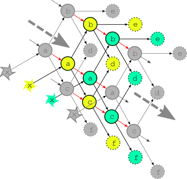
Fig. 6 The complete multi-cycle-point dependency graph. The complete dependency graph for the example suite, assuming the least possible inter-cycle dependence: the models (a, b, and c) depend on their own previous instances. The dashed arrows show connections to previous and subsequent cycle points.

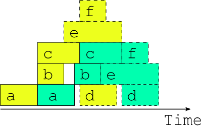
Fig. 7 The optimal two-cycle-point job schedule. The optimal two cycle job schedule when the next cycle’s driving data is available in advance, possible in principle when inter-cycle dependence is handled explicitly.

Fig. 7 shows, in contrast to Fig. 4, the optimal two cycle point job schedule obtained by respecting all inter-cycle dependence. This assumes no delays due to resource contention or otherwise - i.e. every task runs as soon as it is ready to run. The scheduler running this suite must be able to adapt dynamically to external conditions that impact on multi-cycle-point scheduling in the presence of inter-cycle dependence or else, again, risk bringing the system down with dependency violations.

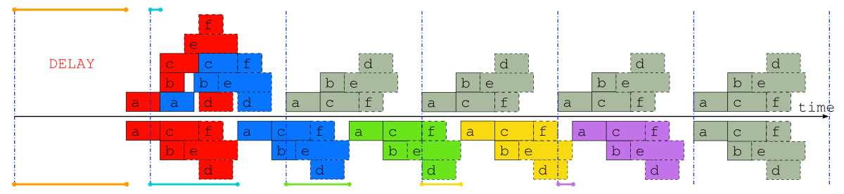
Fig. 8 Comparison of job schedules after a delay. Job schedules for the example suite after a delay of almost one whole cycle point, when inter-cycle dependence is taken into account (above the time axis), and when it is not (below the time axis). The colored lines indicate the time that each cycle point is delayed, and normal “caught up” cycle points are shaded gray.

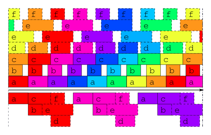
Fig. 9 Optimal job schedule when all external data is available. Job schedules for the example suite in case study mode, or after a long delay, when the external driving data are available many cycle points in advance. Above the time axis is the optimal schedule obtained when the suite is constrained only by its true dependencies, as in Fig. 3, and underneath is the best that can be done, in general, when inter-cycle dependence is ignored.

To further illustrate the potential benefits of proper inter-cycle dependency handling, Fig. 8 shows an operational delay of almost one whole cycle point in a suite with little downtime between cycle points. Above the time axis is the optimal schedule that is possible in principle when inter-cycle dependence is taken into account, and below it is the only safe schedule possible in general when it is ignored. In the former case, even the cycle point immediately after the delay is hardly affected, and subsequent cycle points are all on time, whilst in the latter case it takes five full cycle points to catch up to normal real time operation [1].

Similarly, Fig. 9 shows example suite job schedules for an historical case study, or when catching up after a very long delay; i.e. when the external driving data are available many cycle points in advance. Task a, which as the most upstream model is likely to be a resource intensive atmosphere or ocean model, has no upstream dependence on co-temporal tasks and can therefore run continuously, regardless of how much downstream processing is yet to be completed in its own, or any previous, cycle point (actually, task a does depend on co-temporal task x which waits on the external driving data, but that returns immediately when the data is available in advance, so the result stands). The other models can also cycle continuously or with a short gap between, and some post processing tasks, which have no previous-instance dependence, can run continuously or even overlap (e.g. e in this case). Thus, even for this very simple example suite, tasks from three or four different cycle points can in principle run simultaneously at any given time.

In fact, if our tasks are able to trigger off internal outputs of upstream tasks (message triggers) rather than waiting on full completion, then successive instances of the models could overlap as well (because model restart outputs are generally completed early in the run) for an even more efficient job schedule.

[1]	Note that simply overlapping the single cycle point schedules of Fig. 2 from the same start point would have resulted in dependency violation by task c. of task proxies in the pool.