9. Suite Configuration
Cylc suites are defined in structured, validated, suite.rc files that concisely specify the properties of, and the relationships between, the various tasks managed by the suite. This section of the User Guide deals with the format and content of the suite.rc file, including task definition. Task implementation - what’s required of the real commands, scripts, or programs that do the processing that the tasks represent - is covered in Task Implementation; and task job submission - how tasks are submitted to run - is in Task Job Submission and Management.
9.1. Suite Configuration Directories
A cylc suite configuration directory contains:
- A suite.rc file: this is the suite configuration.
- And any include-files used in it (see below; may be kept in sub-directories).
- A
bin/sub-directory (optional)- For scripts and executables that implement, or are used by, suite tasks.
- Automatically added to
$PATHin task execution environments. - Alternatively, tasks can call external commands, scripts, or programs; or they can be scripted entirely within the suite.rc file.
- A
lib/python/sub-directory (optional)- For custom job submission modules (see Custom Job Submission Methods) and local Python modules imported by custom Jinja2 filters, tests and globals (see Custom Jinja2 Filters, Tests and Globals).
- Any other sub-directories and files - documentation,
control files, etc. (optional)
- Holding everything in one place makes proper suite revision control possible.
- Portable access to files here, for running tasks, is
provided through
$CYLC_SUITE_DEF_PATH(see Task Execution Environment). - Ignored by cylc, but the entire suite configuration directory tree is copied when you copy a suite using cylc commands.
A typical example:
/path/to/my/suite   # suite configuration directory
    suite.rc           # THE SUITE CONFIGURATION FILE
    bin/               # scripts and executables used by tasks
        foo.sh
        bar.sh
        ...
    # (OPTIONAL) any other suite-related files, for example:
    inc/               # suite.rc include-files
        nwp-tasks.rc
        globals.rc
        ...
    doc/               # documentation
    control/           # control files
    ancil/             # ancillary files
    ...
9.2. Suite.rc File Overview
Suite.rc files are an extended-INI format with section nesting.
Embedded template processor expressions may also be used in the file, to programatically generate the final suite configuration seen by cylc. Currently the Jinja2 and EmPy template processors are supported; see Jinja2 and EmPy for examples. In the future cylc may provide a plug-in interface to allow use of other template engines too.
9.2.1. Syntax
The following defines legal suite.rc syntax:
- Items are of the form
item = value. - [Section] headings are enclosed in square brackets.
- Sub-section [[nesting]] is defined by repeated square brackets.
- Sections are closed by the next section heading.
- Comments (line and trailing) follow a hash character:
# - List values are comma-separated.
- Single-line string values can be single-, double-, or un-quoted.
- Multi-line string values are triple-quoted (using single or double quote characters).
- Boolean values are capitalized: True, False.
- Leading and trailing whitespace is ignored.
- Indentation is optional but should be used for clarity.
- Continuation lines follow a trailing backslash:
\ - Duplicate sections add their items to those previously defined under the same section.
- Duplicate items override, except for dependency ``graph`` strings, which are additive.
- Include-files
%include inc/foo.rccan be used as a verbatim inlining mechanism.
Suites that embed templating code (see Jinja2 and EmPy) must process to raw suite.rc syntax.
9.2.2. Include-Files
Cylc has native support for suite.rc include-files, which may help to organize large suites. Inclusion boundaries are completely arbitrary - you can think of include-files as chunks of the suite.rc file simply cut-and-pasted into another file. Include-files may be included multiple times in the same file, and even nested. Include-file paths can be specified portably relative to the suite configuration directory, e.g.:
# include the file $CYLC_SUITE_DEF_PATH/inc/foo.rc:
%include inc/foo.rc
9.2.2.1. Editing Temporarily Inlined Suites
Cylc’s native file inclusion mechanism supports optional inlined editing:
$ cylc edit --inline SUITE
The suite will be split back into its constituent include-files when you
exit the edit session. While editing, the inlined file becomes the
official suite configuration so that changes take effect whenever you save
the file. See cylc prep edit --help for more information.
9.2.3. Syntax Highlighting For Suite Configuration
Cylc comes with syntax files for a number of text editors:
<cylc-dir>/etc/syntax/cylc.vim     # vim
<cylc-dir>/etc/syntax/cylc-mode.el # emacs
<cylc-dir>/etc/syntax/cylc.lang    # gedit (and other gtksourceview programs)
<cylc-dir>/etc/syntax/cylc.xml     # kate
Refer to comments at the top of each file to see how to use them.
9.2.4. Gross File Structure
Cylc suite.rc files consist of a suite title and description followed by configuration items grouped under several top level section headings:
- [cylc] - non task-specific suite configuration
- [scheduling] - determines when tasks are ready to run
- tasks with special behaviour, e.g. clock-trigger tasks
- the dependency graph, which defines the relationships between tasks
- [runtime] - determines how, where, and what to
execute when tasks are ready
- script, environment, job submission, remote hosting, etc.
- suite-wide defaults in the root namespace
- a nested family hierarchy with common properties inherited by related tasks
- [visualization] - suite graph styling
9.2.5. Validation
Cylc suite.rc files are automatically validated against a specification that defines all legal entries, values, options, and defaults. This detects formatting errors, typographic errors, illegal items and illegal values prior to run time. Some values are complex strings that require further parsing by cylc to determine their correctness (this is also done during validation). All legal entries are documented in (Suite.rc Reference).
The validator reports the line numbers of detected errors. Here’s an example showing a section heading with a missing right bracket:
$ cylc validate my.suite
    [[special tasks]
'Section bracket mismatch, line 19'
If the suite.rc file uses include-files cylc view will
show an inlined copy of the suite with correct line numbers
(you can also edit suites in a temporarily inlined state with
cylc edit --inline).
Validation does not check the validity of chosen batch systems.
9.3. Scheduling - Dependency Graphs
The [scheduling] section of a suite.rc file defines the
relationships between tasks in a suite - the information that allows
cylc to determine when tasks are ready to run. The most important
component of this is the suite dependency graph. Cylc graph notation
makes clear textual graph representations that are very concise because
sections of the graph that repeat at different hours of the day, say,
only have to be defined once. Here’s an example with dependencies that
vary depending on the particular cycle point:
[scheduling]
    initial cycle point = 20200401
    final cycle point = 20200405
    [[dependencies]]
        [[[T00,T06,T12,T18]]] # validity (hours)
            graph = """
A => B & C   # B and C trigger off A
A[-PT6H] => A  # Model A restart trigger
                    """
        [[[T06,T18]]] # hours
            graph = "C => X"
Fig. 21 shows the complete suite.rc listing alongside
the suite graph. This is a complete, valid, runnable suite (it will
use default task runtime properties such as script).
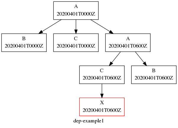
Example Suite
[meta]
    title = "Dependency Example 1"
[cylc]
    UTC mode = True
[scheduling]
    initial cycle point = 20200401
    final cycle point = 20200405
    [[dependencies]]
        [[[T00,T06,T12,T18]]] # validity (hours)
            graph = """
A => B & C   # B and C trigger off A
A[-PT6H] => A  # Model A restart trigger
                    """
        [[[T06,T18]]] # hours
            graph = "C => X"
[visualization]
    initial cycle point = 20200401
    final cycle point = 20200401T06
    [[node attributes]]
        X = "color=red"
9.3.1. Graph String Syntax
Multiline graph strings may contain:
- blank lines
- arbitrary white space
- internal comments: following the
#character - conditional task trigger expressions - see below.
9.3.2. Interpreting Graph Strings
Suite dependency graphs can be broken down into pairs in which the left side (which may be a single task or family, or several that are conditionally related) defines a trigger for the task or family on the right. For instance the “word graph” C triggers off B which triggers off A can be deconstructed into pairs C triggers off B and B triggers off A. In this section we use only the default trigger type, which is to trigger off the upstream task succeeding; see Task Triggering for other available triggers.
In the case of cycling tasks, the triggers defined by a graph string are valid for cycle points matching the list of hours specified for the graph section. For example this graph:
[scheduling]
    [[dependencies]]
        [[[T00,T12]]]
            graph = "A => B"
implies that B triggers off A for cycle points in which the hour matches 00
or 12.
To define inter-cycle dependencies, attach an offset indicator to the left side of a pair:
[scheduling]
    [[dependencies]]
        [[[T00,T12]]]
            graph = "A[-PT12H] => B"
This means B[time] triggers off A[time-PT12H] (12 hours before) for cycle
points with hours matching 00 or 12. time is implicit because
this keeps graphs clean and concise, given that the
majority of tasks will typically
depend only on others with the same cycle point. Cycle point offsets can only
appear on the left of a pair, because a pairs define triggers for the right
task at cycle point time. However, A => B[-PT6H], which is
illegal, can be reformulated as a future trigger
A[+PT6H] => B (see Inter-Cycle Triggers). It is also
possible to combine multiple offsets within a cycle point offset e.g.
[scheduling]
    [[dependencies]]
        [[[T00,T12]]]
            graph = "A[-P1D-PT12H] => B"
This means that B[Time] triggers off A[time-P1D-PT12H] (1 day and 12 hours before).
Triggers can be chained together. This graph:
graph = """A => B  # B triggers off A
           B => C  # C triggers off B"""
is equivalent to this:
graph = "A => B => C"
Each trigger in the graph must be unique but the same task can appear in multiple pairs or chains. Separately defined triggers for the same task have an AND relationship. So this:
graph = """A => X  # X triggers off A
           B => X  # X also triggers off B"""
is equivalent to this:
graph = "A & B => X" # X triggers off A AND B
In summary, the branching tree structure of a dependency graph can be partitioned into lines (in the suite.rc graph string) of pairs or chains, in any way you like, with liberal use of internal white space and comments to make the graph structure as clear as possible.
# B triggers if A succeeds, then C and D trigger if B succeeds:
    graph = "A => B => C & D"
# which is equivalent to this:
    graph = """A => B => C
               B => D"""
# and to this:
    graph = """A => B => D
               B => C"""
# and to this:
    graph = """A => B
               B => C
               B => D"""
# and it can even be written like this:
    graph = """A => B # blank line follows:

               B => C # comment ...
               B => D"""
9.3.2.1. Splitting Up Long Graph Lines
It is not necessary to use the general line continuation marker
\ to split long graph lines. Just break at dependency arrows,
or split long chains into smaller ones. This graph:
graph = "A => B => C"
is equivalent to this:
graph = """A => B =>
           C"""
and also to this:
graph = """A => B
           B => C"""
9.3.3. Graph Types
A suite configuration can contain multiple graph strings that are combined to generate the final graph.
9.3.3.1. One-off (Non-Cycling)
Fig. 22 shows a small suite of one-off non-cycling
tasks; these all share a single cycle point (1) and don’t spawn
successors (once they’re all finished the suite just exits). The integer
1 attached to each graph node is just an arbitrary label here.
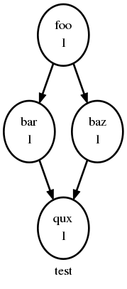
One-off (Non-Cycling) Tasks.
[meta]
    title = some one-off tasks
[scheduling]
    [[dependencies]]
        graph = "foo => bar & baz => qux"
9.3.3.2. Cycling Graphs
For cycling tasks the graph section heading defines a sequence of cycle points for which the subsequent graph section is valid. Fig. 23 shows a small suite of cycling tasks.
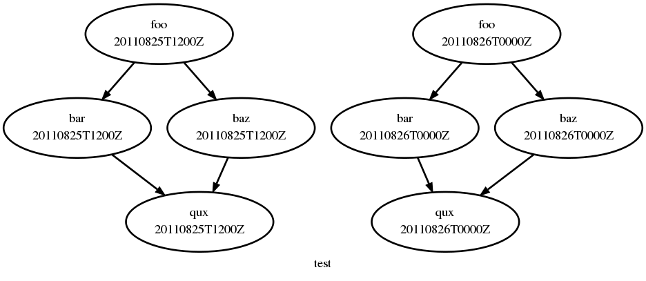
Cycling Tasks.
[meta]
    title = some cycling tasks
# (no dependence between cycle points)
[scheduling]
    [[dependencies]]
        [[[T00,T12]]]
            graph = "foo => bar & baz => qux"
9.3.4. Graph Section Headings
Graph section headings define recurrence expressions, the graph within a graph section heading defines a workflow at each point of the recurrence. For example in the following scenario:
[scheduling]
    [[dependencies]]
        [[[ T06 ]]]  # A graph section heading
            graph = foo => bar
T06 means “Run every day starting at 06:00 after the
initial cycle point”. Cylc allows you to start (or end) at any particular
time, repeat at whatever frequency you like, and even optionally limit the
number of repetitions.
Graph section heading can also be used with integer cycling see Integer Cycling.
9.3.4.1. Syntax Rules
Date-time cycling information is made up of a starting date-time, an interval, and an optional limit.
The time is assumed to be in the local time zone unless you set
[cylc]cycle point time zone or [cylc]UTC mode. The
calendar is assumed to be the proleptic Gregorian calendar unless you set
[scheduling]cycling mode.
The syntax for representations is based on the ISO 8601 date-time standard.
This includes the representation of date-time, interval. What we
define for cylc’s cycling syntax is our own optionally-heavily-condensed form
of ISO 8601 recurrence syntax. The most common full form is:
R[limit?]/[date-time]/[interval]. However, we allow omitting
information that can be guessed from the context (rules below). This means
that it can be written as:
R[limit?]/[date-time]
R[limit?]//[interval]
[date-time]/[interval]
R[limit?] # Special limit of 1 case
[date-time]
[interval]
with example graph headings for each form being:
[[[ R5/T00 ]]]           # Run 5 times at 00:00 every day
[[[ R//PT1H ]]]          # Run every hour (Note the R// is redundant)
[[[ 20000101T00Z/P1D ]]] # Run every day starting at 00:00 1st Jan 2000
[[[ R1 ]]]               # Run once at the initial cycle point
[[[ R1/20000101T00Z ]]]  # Run once at 00:00 1st Jan 2000
[[[ P1Y ]]]              # Run every year
Note
T00 is an example of [date-time], with an
inferred 1 day period and no limit.
Where some or all date-time information is omitted, it is inferred to
be relative to the initial date-time cycle point. For example, T00
by itself would mean the next occurrence of midnight that follows, or is, the
initial cycle point. Entering +PT6H would mean 6 hours after the
initial cycle point. Entering -P1D would mean 1 day before the
initial cycle point. Entering no information for the date-time implies
the initial cycle point date-time itself.
Where the interval is omitted and some (but not all) date-time
information is omitted, it is inferred to be a single unit above
the largest given specific date-time unit. For example, the largest
given specific unit in T00 is hours, so the inferred interval is
1 day (daily), P1D.
Where the limit is omitted, unlimited cycling is assumed. This will be bounded by the final cycle point’s date-time if given.
Another supported form of ISO 8601 recurrence is:
R[limit?]/[interval]/[date-time]. This form uses the
date-time as the end of the cycling sequence rather than the start.
For example, R3/P5D/20140430T06 means:
20140420T06
20140425T06
20140430T06
This kind of form can be used for specifying special behaviour near the end of the suite, at the final cycle point’s date-time. We can also represent this in cylc with a collapsed form:
R[limit?]/[interval]
R[limit?]//[date-time]
[interval]/[date-time]
So, for example, you can write:
[[[ R1//+P0D ]]]  # Run once at the final cycle point
[[[ R5/P1D ]]]    # Run 5 times, every 1 day, ending at the final
                  # cycle point
[[[ P2W/T00 ]]]   # Run every 2 weeks ending at 00:00 following
                  # the final cycle point
[[[ R//T00 ]]]    # Run every 1 day ending at 00:00 following the
                  # final cycle point
9.3.4.2. Referencing The Initial And Final Cycle Points
For convenience the caret and dollar symbols may be used as shorthand for the initial and final cycle points. Using this shorthand you can write:
[[[ R1/^+PT12H ]]]  # Repeat once 12 hours after the initial cycle point
                    # R[limit]/[date-time]
                    # Equivalent to [[[ R1/+PT12H ]]]
[[[ R1/$ ]]]        # Repeat once at the final cycle point
                    # R[limit]/[date-time]
                    # Equivalent to [[[ R1//+P0D ]]]
[[[ $-P2D/PT3H ]]]  # Repeat 3 hourly starting two days before the
                    # [date-time]/[interval]
                    # final cycle point
Note
There can be multiple ways to write the same headings, for instance the following all run once at the final cycle point:
[[[ R1/P0Y ]]]      # R[limit]/[interval]
[[[ R1/P0Y/$ ]]]    # R[limit]/[interval]/[date-time]
[[[ R1/$ ]]]        # R[limit]/[date-time]
9.3.4.3. Excluding Dates
Date-times can be excluded from a recurrence by an exclamation mark for
example [[[ PT1D!20000101 ]]] means run daily except on the
first of January 2000.
This syntax can be used to exclude one or multiple date-times from a
recurrence. Multiple date-times are excluded using the syntax
[[[ PT1D!(20000101,20000102,...) ]]]. All date-times listed within
the parentheses after the exclamation mark will be excluded.
Note
The ^ and $ symbols (shorthand for the initial
and final cycle points) are both date-times so [[[ T12!$-PT1D ]]]
is valid.
If using a run limit in combination with an exclusion, the heading might not
run the number of times specified in the limit. For example in the following
suite foo will only run once as its second run has been excluded.
[scheduling]
    initial cycle point = 20000101T00Z
    final cycle point = 20000105T00Z
    [[dependencies]]
        [[[ R2/P1D!20000102 ]]]
            graph = foo
9.3.4.4. Advanced exclusion syntax
In addition to excluding isolated date-time points or lists of date-time points from recurrences, exclusions themselves may be date-time recurrence sequences. Any partial date-time or sequence given after the exclamation mark will be excluded from the main sequence.
For example, partial date-times can be excluded using the syntax:
[[[ PT1H ! T12 ]]]          # Run hourly but not at 12:00 from the initial
                            # cycle point.
[[[ T-00 ! (T00, T06, T12, T18) ]]]   # Run hourly but not at 00:00, 06:00,
                                      # 12:00, 18:00.
[[[ PT5M ! T-15 ]]]         # Run 5-minutely but not at 15 minutes past the
                            # hour from the initial cycle point.
[[[ T00 ! W-1T00 ]]]        # Run daily at 00:00 except on Mondays.
It is also valid to use sequences for exclusions. For example:
[[[ PT1H ! PT6H ]]]         # Run hourly from the initial cycle point but
                            # not 6-hourly from the initial cycle point.
[[[ T-00 ! PT6H ]]]         # Run hourly on the hour but not 6-hourly
                            # on the hour.
    # Same as [[[ T-00 ! T-00/PT6H ]]] (T-00 context is implied)
    # Same as [[[ T-00 ! (T00, T06, T12, T18) ]]]
    # Same as [[[ PT1H ! (T00, T06, T12, T18) ]]] Initial cycle point dependent

[[[ T12 ! T12/P15D ]]]      # Run daily at 12:00 except every 15th day.

[[[ R/^/P1H ! R5/20000101T00/P1D ]]]    # Any valid recurrence may be used to
                                        # determine exclusions. This example
                                        # translates to: Repeat every hour from
                                        # the initial cycle point, but exclude
                                        # 00:00 for 5 days from the 1st January
                                        # 2000.
You can combine exclusion sequences and single point exclusions within a comma separated list enclosed in parentheses:
[[[ T-00 ! (20000101T07, PT2H) ]]]      # Run hourly on the hour but not at 07:00
                                        # on the 1st Jan, 2000 and not 2-hourly
                                        # on the hour.
9.3.4.5. How Multiple Graph Strings Combine
For a cycling graph with multiple validity sections for different hours of the day, the different sections add to generate the complete graph. Different graph sections can overlap (i.e. the same hours may appear in multiple section headings) and the same tasks may appear in multiple sections, but individual dependencies should be unique across the entire graph. For example, the following graph defines a duplicate prerequisite for task C:
[scheduling]
    [[dependencies]]
        [[[T00,T06,T12,T18]]]
            graph = "A => B => C"
        [[[T06,T18]]]
            graph = "B => C => X"
            # duplicate prerequisite: B => C already defined at T06, T18
This does not affect scheduling, but for the sake of clarity and brevity the graph should be written like this:
[scheduling]
    [[dependencies]]
        [[[T00,T06,T12,T18]]]
            graph = "A => B => C"
        [[[T06,T18]]]
            # X triggers off C only at 6 and 18 hours
            graph = "C => X"
9.3.4.6. Advanced Examples
The following examples show the various ways of writing graph headings in cylc.
[[[ R1 ]]]         # Run once at the initial cycle point
[[[ P1D ]]]        # Run every day starting at the initial cycle point
[[[ PT5M ]]]       # Run every 5 minutes starting at the initial cycle
                   # point
[[[ T00/P2W ]]]    # Run every 2 weeks starting at 00:00 after the
                   # initial cycle point
[[[ +P5D/P1M ]]]   # Run every month, starting 5 days after the initial
                   # cycle point
[[[ R1/T06 ]]]     # Run once at 06:00 after the initial cycle point
[[[ R1/P0Y ]]]     # Run once at the final cycle point
[[[ R1/$ ]]]       # Run once at the final cycle point (alternative
                   # form)
[[[ R1/$-P3D ]]]   # Run once three days before the final cycle point
[[[ R3/T0830 ]]]   # Run 3 times, every day at 08:30 after the initial
                   # cycle point
[[[ R3/01T00 ]]]   # Run 3 times, every month at 00:00 on the first
                   # of the month after the initial cycle point
[[[ R5/W-1/P1M ]]] # Run 5 times, every month starting on Monday
                   # following the initial cycle point
[[[ T00!^ ]]]      # Run at the first occurrence of T00 that isn't the
                   # initial cycle point
[[[ PT1D!20000101 ]]]  # Run every day days excluding 1st Jan 2000
[[[ 20140201T06/P1D ]]]    # Run every day starting at 20140201T06
[[[ R1/min(T00,T06,T12,T18) ]]]  # Run once at the first instance
                                 # of either T00, T06, T12 or T18
                                 # starting at the initial cycle
                                 # point
9.3.4.7. Advanced Starting Up
Dependencies that are only valid at the initial cycle point can be written
using the R1 notation (e.g. as in Initial Non-Repeating (R1) Tasks.
For example:
[cylc]
    UTC mode = True
[scheduling]
    initial cycle point = 20130808T00
    final cycle point = 20130812T00
    [[dependencies]]
        [[[R1]]]
            graph = "prep => foo"
        [[[T00]]]
            graph = "foo[-P1D] => foo => bar"
In the example above, R1 implies R1/20130808T00, so
prep only runs once at that cycle point (the initial cycle point).
At that cycle point, foo will have a dependence on
prep - but not at subsequent cycle points.
However, it is possible to have a suite that has multiple effective initial
cycles - for example, one starting at T00 and another starting
at T12. What if they need to share an initial task?
Let’s suppose that we add the following section to the suite example above:
[cylc]
    UTC mode = True
[scheduling]
    initial cycle point = 20130808T00
    final cycle point = 20130812T00
    [[dependencies]]
        [[[R1]]]
            graph = "prep => foo"
        [[[T00]]]
            graph = "foo[-P1D] => foo => bar"
        [[[T12]]]
            graph = "baz[-P1D] => baz => qux"
We’ll also say that there should be a starting dependence between
prep and our new task baz - but we still want to have
a single prep task, at a single cycle.
We can write this using a special case of the task[-interval] syntax -
if the interval is null, this implies the task at the initial cycle point.
For example, we can write our suite like Fig. 24.
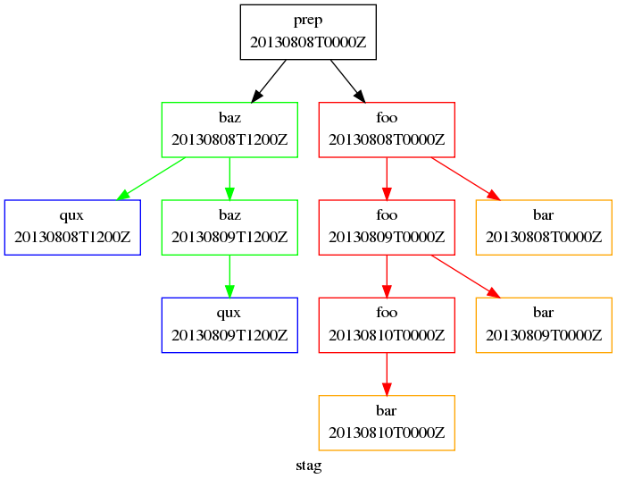
Staggered Start Suite
[cylc]
    UTC mode = True
[scheduling]
    initial cycle point = 20130808T00
    final cycle point = 20130812T00
    [[dependencies]]
        [[[R1]]]
            graph = "prep"
        [[[R1/T00]]]
# ^ implies the initial cycle point:
     graph = "prep[^] => foo"
        [[[R1/T12]]]
# ^ is initial cycle point, as above:
     graph = "prep[^] => baz"
        [[[T00]]]
     graph = "foo[-P1D] => foo => bar"
        [[[T12]]]
     graph = "baz[-P1D] => baz => qux"
[visualization]
    initial cycle point = 20130808T00
    final cycle point = 20130810T00
    [[node attributes]]
        foo = "color=red"
        bar = "color=orange"
        baz = "color=green"
        qux = "color=blue"
This neatly expresses what we want - a task running at the initial cycle point that has one-off dependencies with other task sets at different cycles.
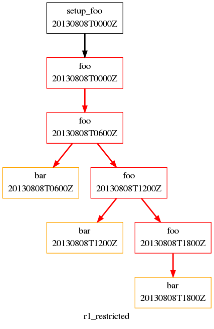
Restricted First Cycle Point Suite
[cylc]
    UTC mode = True
[scheduling]
    initial cycle point = 20130808T00
    final cycle point = 20130808T18
    [[dependencies]]
        [[[R1]]]
            graph = "setup_foo => foo"
        [[[+PT6H/PT6H]]]
            graph = """
                foo[-PT6H] => foo
                foo => bar
            """
[visualization]
    initial cycle point = 20130808T00
    final cycle point = 20130808T18
    [[node attributes]]
        foo = "color=red"
        bar = "color=orange"
A different kind of requirement is displayed in Fig. 25. Usually, we want to specify additional tasks and dependencies at the initial cycle point. What if we want our first cycle point to be entirely special, with some tasks missing compared to subsequent cycle points?
In Fig. 25, bar will not be run at the initial
cycle point, but will still run at subsequent cycle points.
[[[+PT6H/PT6H]]] means start at +PT6H (6 hours after
the initial cycle point) and then repeat every PT6H (6 hours).
Some suites may have staggered start-up sequences where different tasks need
running once but only at specific cycle points, potentially due to differing
data sources at different cycle points with different possible initial cycle
points. To allow this cylc provides a min( ) function that can be
used as follows:
[cylc]
    UTC mode = True
[scheduling]
    initial cycle point = 20100101T03
    [[dependencies]]
        [[[R1/min(T00,T12)]]]
            graph = "prep1 => foo"
        [[[R1/min(T06,T18)]]]
            graph = "prep2 => foo"
        [[[T00,T06,T12,T18]]]
            graph = "foo => bar"
In this example the initial cycle point is 20100101T03, so the
prep1 task will run once at 20100101T12 and the
prep2 task will run once at 20100101T06 as these are
the first cycle points after the initial cycle point in the respective
min( ) entries.
9.3.4.8. Integer Cycling
In addition to non-repeating and date-time cycling workflows, cylc can do integer cycling for repeating workflows that are not date-time based.
To construct an integer cycling suite, set
[scheduling]cycling mode = integer, and specify integer values for
the initial and (optional) final cycle points. The notation for intervals,
offsets, and recurrences (sequences) is similar to the date-time cycling
notation, except for the simple integer values.
The full integer recurrence expressions supported are:
Rn/start-point/interval # e.g. R3/1/P2Rn/interval/end-point # e.g. R3/P2/9
But, as for date-time cycling, sequence start and end points can be omitted where suite initial and final cycle points can be assumed. Some examples:
[[[ R1 ]]]        # Run once at the initial cycle point
                  # (short for R1/initial-point/?)
[[[ P1 ]]]        # Repeat with step 1 from the initial cycle point
                  # (short for R/initial-point/P1)
[[[ P5 ]]]        # Repeat with step 5 from the initial cycle point
                  # (short for R/initial-point/P5)
[[[ R2//P2 ]]]    # Run twice with step 3 from the initial cycle point
                  # (short for R2/initial-point/P2)
[[[ R/+P1/P2 ]]]  # Repeat with step 2, from 1 after the initial cycle point
[[[ R2/P2 ]]]     # Run twice with step 2, to the final cycle point
                  # (short for R2/P2/final-point)
[[[ R1/P0 ]]]     # Run once at the final cycle point
                  # (short for R1/P0/final-point)
9.3.4.8.1. Example
The tutorial illustrates integer cycling in Integer Cycling, and
<cylc-dir>/etc/examples/satellite/ is a
self-contained example of a realistic use for integer cycling. It simulates
the processing of incoming satellite data: each new dataset arrives after a
random (as far as the suite is concerned) interval, and is labeled by an
arbitrary (as far as the suite is concerned) ID in the filename. A task called
get_data at the top of the repeating workflow waits on the next
dataset and, when it finds one, moves it to a cycle-point-specific shared
workspace for processing by the downstream tasks. When get_data.1
finishes, get_data.2 triggers and begins waiting for the next
dataset at the same time as the downstream tasks in cycle point 1 are
processing the first one, and so on. In this way multiple datasets can be
processed at once if they happen to come in quickly. A single shutdown task
runs at the end of the final cycle to collate results. The suite graph is
shown in Fig. 26.
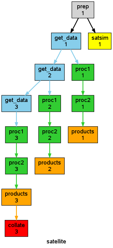
Fig. 26 The etc/examples/satellite integer suite.
9.3.4.8.2. Advanced Integer Cycling Syntax
The same syntax used to reference the initial and final cycle points (introduced in Referencing The Initial And Final Cycle Points) for use with date-time cycling can also be used for integer cycling. For example you can write:
[[[ R1/^ ]]]     # Run once at the initial cycle point
[[[ R1/$ ]]]     # Run once at the final cycle point
[[[ R3/^/P2 ]]]  # Run three times with step two starting at the
                 # initial cycle point
Likewise the syntax introduced in Excluding Dates for excluding a particular point from a recurrence also works for integer cycling. For example:
[[[ R/P4!8 ]]]       # Run with step 4, to the final cycle point
                     # but not at point 8
[[[ R3/3/P2!5 ]]]    # Run with step 2 from point 3 but not at
                     # point 5
[[[ R/+P1/P6!14 ]]]  # Run with step 6 from 1 step after the
                     # initial cycle point but not at point 14
Multiple integer exclusions are also valid in the same way as the syntax in Excluding Dates. Integer exclusions may be a list of single integer points, an integer sequence, or a combination of both:
[[[ R/P1!(2,3,7) ]]]  # Run with step 1 to the final cycle point,
                      # but not at points 2, 3, or 7.
[[[ P1 ! P2 ]]]       # Run with step 1 from the initial to final
                      # cycle point, skipping every other step from
                      # the initial cycle point.
[[[ P1 ! +P1/P2 ]]]   # Run with step 1 from the initial cycle point,
                      # excluding every other step beginning one step
                      # after the initial cycle point.
[[[ P1 !(P2,6,8) ]]]  # Run with step 1 from the initial cycle point,
                      # excluding every other step, and also excluding
                      # steps 6 and 8.
9.3.5. Task Triggering
A task is said to “trigger” when it submits its job to run, as soon as all of
its dependencies (also known as its separate “triggers”) are met. Tasks can
be made to trigger off of the state of other tasks (indicated by a
:state qualifier on the upstream task (or family)
name in the graph) and, and off the clock, and arbitrary external events.
External triggering is relatively more complicated, and is documented separately in External Triggers.
9.3.5.1. Success Triggers
The default, with no trigger type specified, is to trigger off the upstream task succeeding:
# B triggers if A SUCCEEDS:
    graph = "A => B"
For consistency and completeness, however, the success trigger can be explicit:
# B triggers if A SUCCEEDS:
    graph = "A => B"
# or:
    graph = "A:succeed => B"
9.3.5.2. Failure Triggers
To trigger off the upstream task reporting failure:
# B triggers if A FAILS:
    graph = "A:fail => B"
Suicide triggers can be used to remove task B here if
A does not fail, see Suicide Triggers.
9.3.5.3. Start Triggers
To trigger off the upstream task starting to execute:
# B triggers if A STARTS EXECUTING:
    graph = "A:start => B"
This can be used to trigger tasks that monitor other tasks once they
(the target tasks) start executing. Consider a long-running forecast model,
for instance, that generates a sequence of output files as it runs. A
postprocessing task could be launched with a start trigger on the model
(model:start => post) to process the model output as it
becomes available. Note, however, that there are several alternative
ways of handling this scenario: both tasks could be triggered at the
same time (foo => model & post), but depending on
external queue delays this could result in the monitoring task starting
to execute first; or a different postprocessing task could be
triggered off a message output for each data file
(model:out1 => post1 etc.; see Message Triggers), but this
may not be practical if the
number of output files is large or if it is difficult to add cylc
messaging calls to the model.
9.3.5.4. Finish Triggers
To trigger off the upstream task succeeding or failing, i.e. finishing one way or the other:
# B triggers if A either SUCCEEDS or FAILS:
    graph = "A | A:fail => B"
# or
    graph = "A:finish => B"
9.3.5.5. Message Triggers
Tasks can also trigger off custom output messages. These must be registered in
the [runtime] section of the emitting task, and reported using the
cylc message command in task scripting. The graph trigger notation
refers to the item name of the registered output message.
The example suite <cylc-dir>/etc/examples/message-triggers illustrates
message triggering.
[meta]
    title = "test suite for cylc-6 message triggers"

[scheduling]
    initial cycle point = 20140801T00
    final cycle point = 20141201T00
    [[dependencies]]
        [[[P2M]]]
           graph = """foo:out1 => bar
                      foo[-P2M]:out2 => baz"""
[runtime]
    [[foo]]
        script = """
sleep 5
cylc message -- "${CYLC_SUITE_NAME}" "${CYLC_TASK_JOB}" "file 1 done"
sleep 10
cylc message -- "${CYLC_SUITE_NAME}" "${CYLC_TASK_JOB}" "file 2 done"
sleep 10"""
        [[[outputs]]]
            out1 = "file 1 done"
            out2 = "file 2 done"
    [[bar, baz]]
        script = sleep 10
9.3.5.6. Job Submission Triggers
It is also possible to trigger off a task submitting, or failing to submit:
# B triggers if A submits successfully:
    graph = "A:submit => B"
# D triggers if C fails to submit successfully:
    graph = "C:submit-fail => D"
A possible use case for submit-fail triggers: if a task goes into the submit-failed state, possibly after several job submission retries, another task that inherits the same runtime but sets a different job submission method and/or host could be triggered to, in effect, run the same job on a different platform.
9.3.5.7. Conditional Triggers
AND operators (&) can appear on both sides of an arrow. They
provide a concise alternative to defining multiple triggers separately:
# 1/ this:
    graph = "A & B => C"
# is equivalent to:
    graph = """A => C
               B => C"""
# 2/ this:
    graph = "A => B & C"
# is equivalent to:
    graph = """A => B
               A => C"""
# 3/ and this:
    graph = "A & B => C & D"
# is equivalent to this:
    graph = """A => C
               B => C
               A => D
               B => D"""
OR operators (|) which result in true conditional triggers,
can only appear on the left [1] :
# C triggers when either A or B finishes:
    graph = "A | B => C"
Forecasting suites typically have simple conditional triggering requirements, but any valid conditional expression can be used, as shown in Fig. 27 (conditional triggers are plotted with open arrow heads).
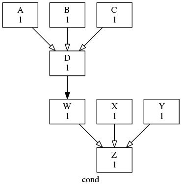
Conditional triggers, which are plotted with open arrow heads.
        graph = """
# D triggers if A or (B and C) succeed
A | B & C => D
# just to align the two graph sections
D => W
# Z triggers if (W or X) and Y succeed
(W|X) & Y => Z
                """
9.3.5.8. Suicide Triggers
Suicide triggers take tasks out of the suite. This can be used for
automated failure recovery. The suite.rc listing and accompanying
graph in Fig. 28 show how to define a chain of failure
recovery tasks that trigger if they’re needed but
otherwise remove themselves from the
suite (you can run the AutoRecover.async example suite to see how
this works). The dashed graph edges ending in solid dots indicate
suicide triggers, and the open arrowheads indicate conditional triggers
as usual. Suicide triggers are ignored by default in the graph view, unless
you toggle them on with View -> Options ->
Ignore Suicide Triggers.
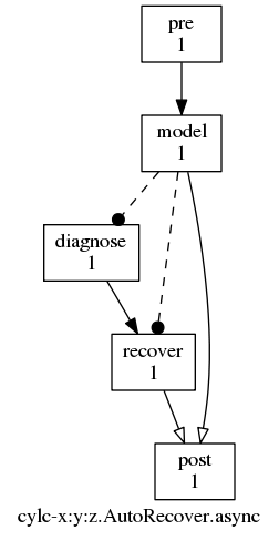
Automated failure recovery via suicide triggers.
[meta]
    title = automated failure recovery
    description = """
Model task failure triggers diagnosis
and recovery tasks, which take themselves
out of the suite if model succeeds. Model
post processing triggers off model OR
recovery tasks.
              """
[scheduling]
    [[dependencies]]
        graph = """
pre => model
model:fail => diagnose => recover
model => !diagnose & !recover
model | recover => post
                """
[runtime]
    [[model]]
        # UNCOMMENT TO TEST FAILURE:
        # script = /bin/false
Note
Multiple suicide triggers combine in the same way as other triggers, so this:
foo => !baz
bar => !baz
is equivalent to this:
foo & bar => !baz
i.e. both foo and bar must succeed for
baz to be taken out of the suite. If you really want a task
to be taken out if any one of several events occurs then be careful to
write it that way:
foo | bar => !baz
Warning
A word of warning on the meaning of “bare suicide triggers”. Consider the following suite:
[scheduling]
    [[dependencies]]
        graph = "foo => !bar"
Task bar has a suicide trigger but no normal prerequisites
(a suicide trigger is not a task triggering prerequisite, it is a task
removal prerequisite) so this is entirely equivalent to:
[scheduling]
    [[dependencies]]
        graph = """
            foo & bar
           foo => !bar
                """
In other words both tasks will trigger immediately, at the same time,
and then bar will be removed if foo succeeds.
If an active task proxy (currently in the submitted or running states) is removed from the suite by a suicide trigger, a warning will be logged.
9.3.5.9. Family Triggers
Families defined by the namespace inheritance hierarchy (Runtime - Task Configuration) can be used in the graph trigger whole groups of tasks at the same time (e.g. forecast model ensembles and groups of tasks for processing different observation types at the same time) and for triggering downstream tasks off families as a whole. Higher level families, i.e. families of families, can also be used, and are reduced to the lowest level member tasks.
Note
Tasks can also trigger off individual family members if necessary.
To trigger an entire task family at once:
[scheduling]
    [[dependencies]]
        graph = "foo => FAM"
[runtime]
    [[FAM]]    # a family (because others inherit from it)
    [[m1,m2]]  # family members (inherit from namespace FAM)
        inherit = FAM
This is equivalent to:
[scheduling]
    [[dependencies]]
        graph = "foo => m1 & m2"
[runtime]
    [[FAM]]
    [[m1,m2]]
        inherit = FAM
To trigger other tasks off families we have to specify whether to triggering off all members starting, succeeding, failing, or finishing, or off any members (doing the same). Legal family triggers are thus:
[scheduling]
    [[dependencies]]
        graph = """
      # all-member triggers:
    FAM:start-all => one
    FAM:succeed-all => one
    FAM:fail-all => one
    FAM:finish-all => one
      # any-member triggers:
    FAM:start-any => one
    FAM:succeed-any => one
    FAM:fail-any => one
    FAM:finish-any => one
                """
Here’s how to trigger downstream processing after if one or more family members succeed, but only after all members have finished (succeeded or failed):
[scheduling]
    [[dependencies]]
        graph = """
    FAM:finish-all & FAM:succeed-any => foo
                """
9.3.5.10. Efficient Inter-Family Triggering
While cylc allows writing dependencies between two families it is important to
consider the number of dependencies this will generate. In the following
example, each member of FAM2 has dependencies pointing at all the
members of FAM1.
[scheduling]
    [[dependencies]]
        graph = """
    FAM1:succeed-any => FAM2
                """
Expanding this out, you generate N * M dependencies, where
N is the number of members of FAM1 and M is
the number of members of FAM2. This can result in high memory use
as the number of members of these families grows, potentially rendering the
suite impractical for running on some systems.
You can greatly reduce the number of dependencies generated in these situations
by putting dummy tasks in the graphing to represent the state of the family you
want to trigger off. For example, if FAM2 should trigger off any
member of FAM1 succeeding you can create a dummy task
FAM1_succeed_any_marker and place a dependency on it as follows:
[scheduling]
    [[dependencies]]
        graph = """
    FAM1:succeed-any => FAM1_succeed_any_marker => FAM2
                """
[runtime]
# ...
    [[FAM1_succeed_any_marker]]
        script = true
# ...
This graph generates only N + M dependencies, which takes
significantly less memory and CPU to store and evaluate.
9.3.5.11. Inter-Cycle Triggers
Typically most tasks in a suite will trigger off others in the same cycle point, but some may depend on others with other cycle points. This notably applies to warm-cycled forecast models, which depend on their own previous instances (see below); but other kinds of inter-cycle dependence are possible too [2] . Here’s how to express this kind of relationship in cylc:
[dependencies]
    [[PT6H]]
        # B triggers off A in the previous cycle point
        graph = "A[-PT6H] => B"
inter-cycle and trigger type (or message trigger) notation can be combined:
# B triggers if A in the previous cycle point fails:
graph = "A[-PT6H]:fail => B"
At suite start-up inter-cycle triggers refer to a previous cycle point that does not exist. This does not cause the dependent task to wait indefinitely, however, because cylc ignores triggers that reach back beyond the initial cycle point. That said, the presence of an inter-cycle trigger does normally imply that something special has to happen at start-up. If a model depends on its own previous instance for restart files, for instance, then an initial set of restart files has to be generated somehow or the first model task will presumably fail with missing input files. There are several ways to handle this in cylc using different kinds of one-off (non-cycling) tasks that run at suite start-up. They are illustrated in Inter-Cycle Triggers; to summarize here briefly:
R1tasks (recommended):[scheduling] [[dependencies]] [[[R1]]] graph = "prep" [[[R1/T00,R1/T12]]] graph = "prep[^] => foo" [[[T00,T12]]] graph = "foo[-PT12H] => foo => bar"
R1, or R1/date-time tasks are the recommended way to
specify unusual start up conditions. They allow you to specify a clean
distinction between the dependencies of initial cycles and the dependencies
of the subsequent cycles.
Initial tasks can be used for real model cold-start processes, whereby a warm-cycled model at any given cycle point can in principle have its inputs satisfied by a previous instance of itself, or by an initial task with (nominally) the same cycle point.
In effect, the R1 task masquerades as the previous-cycle-point trigger
of its associated cycling task. At suite start-up initial tasks will
trigger the first cycling tasks, and thereafter the inter-cycle trigger
will take effect.
If a task has a dependency on another task in a different cycle point, the
dependency can be written using the [offset] syntax such as
[-PT12H] in foo[-PT12H] => foo. This means that
foo at the current cycle point depends on a previous instance of
foo at 12 hours before the current cycle point. Unlike the
cycling section headings (e.g. [[[T00,T12]]]), dependencies
assume that relative times are relative to the current cycle point, not the
initial cycle point.
However, it can be useful to have specific dependencies on tasks at or near
the initial cycle point. You can switch the context of the offset to be
the initial cycle point by using the caret symbol: ^.
For example, you can write foo[^] to mean foo at the initial
cycle point, and foo[^+PT6H] to mean foo 6 hours after the initial
cycle point. Usually, this kind of dependency will only apply in a limited
number of cycle points near the start of the suite, so you may want to write
it in R1-based cycling sections. Here’s the example inter-cycle
R1 suite from above again.
[scheduling]
    [[dependencies]]
        [[[R1]]]
            graph = "prep"
        [[[R1/T00,R1/T12]]]
            graph = "prep[^] => foo"
        [[[T00,T12]]]
            graph = "foo[-PT12H] => foo => bar"
You can see there is a dependence on the initial R1 task
prep for foo at the first T00 cycle point,
and at the first T12 cycle point. Thereafter, foo just
depends on its previous (12 hours ago) instance.
Finally, it is also possible to have a dependency on a task at a specific cycle point.
[scheduling]
    [[dependencies]]
        [[[R1/20200202]]]
            graph = "baz[20200101] => qux"
However, in a long running suite, a repeating cycle should avoid having a
dependency on a task with a specific cycle point (including the initial cycle
point) - as it can currently cause performance issue. In the following example,
all instances of qux will depend on baz.20200101, which
will never be removed from the task pool:
[scheduling]
    initial cycle point = 2010
    [[dependencies]]
        # Can cause performance issue!
        [[[P1D]]]
            graph = "baz[20200101] => qux"
9.3.5.12. Special Sequential Tasks
Tasks that depend on their own previous-cycle instance can be declared as sequential:
[scheduling]
    [[special tasks]]
        # foo depends on its previous instance:
        sequential = foo  # deprecated - see below!
    [[dependencies]]
        [[[T00,T12]]]
            graph = "foo => bar"
The sequential declaration is deprecated however, in favor of explicit inter-cycle triggers which clearly expose the same scheduling behaviour in the graph:
[scheduling]
    [[dependencies]]
        [[[T00,T12]]]
            # foo depends on its previous instance:
            graph = "foo[-PT12H] => foo => bar"
The sequential declaration is arguably convenient in one unusual situation though: if a task has a non-uniform cycling sequence then multiple explicit triggers,
[scheduling]
    [[dependencies]]
        [[[T00,T03,T11]]]
            graph = "foo => bar"
        [[[T00]]]
            graph = "foo[-PT13H] => foo"
        [[[T03]]]
            graph = "foo[-PT3H] => foo"
        [[[T11]]]
            graph = "foo[-PT8H] => foo"
can be replaced by a single sequential declaration,
[scheduling]
    [[special tasks]]
        sequential = foo
    [[dependencies]]
        [[[T00,T03,T11]]]
            graph = "foo => bar"
9.3.5.13. Future Triggers
Cylc also supports inter-cycle triggering off tasks “in the future” (with respect to cycle point - which has no bearing on wall-clock job submission time unless the task has a clock trigger):
[[dependencies]]
    [[[T00,T06,T12,T18]]]
        graph = """
    # A runs in this cycle:
            A
    # B in this cycle triggers off A in the next cycle.
            A[PT6H] => B
        """
Future triggers present a problem at suite shutdown rather than at start-up.
Here, B at the final cycle point wants to trigger off an instance
of A that will never exist because it is beyond the suite stop
point. Consequently Cylc prevents tasks from spawning successors that depend on
other tasks beyond the final point.
9.3.5.14. Clock Triggers
Note
Please read External Triggers (External Triggers) before using the older clock triggers described in this section.
By default, date-time cycle points are not connected to the real time “wall clock”. They are just labels that are passed to task jobs (e.g. to initialize an atmospheric model run with a particular date-time value). In real time cycling systems, however, some tasks - typically those near the top of the graph in each cycle - need to trigger at or near the time when their cycle point is equal to the real clock date-time.
So clock triggers allow tasks to trigger at (or after, depending on other triggers) a wall clock time expressed as an offset from cycle point:
[scheduling]
    [[special tasks]]
        clock-trigger = foo(PT2H)
    [[dependencies]]
        [[[T00]]]
            graph = foo
Here, foo[2015-08-23T00] would trigger (other dependencies allowing)
when the wall clock time reaches 2015-08-23T02. Clock-trigger
offsets are normally positive, to trigger some time after the wall-clock
time is equal to task cycle point.
Clock-triggers have no effect on scheduling if a suite is running sufficiently far behind the clock (e.g. after a delay, or because it is processing archived historical data) that the trigger times, which are relative to task cycle point, have already passed.
9.3.5.15. Clock-Expire Triggers
Tasks can be configured to expire - i.e. to skip job submission and
enter the expired state - if they are too far behind the wall clock when
they become ready to run, and other tasks can trigger off this. As a possible
use case, consider a cycling task that copies the latest of a set of files to
overwrite the previous set: if the task is delayed by more than one cycle there
may be no point in running it because the freshly copied files will just be
overwritten immediately by the next task instance as the suite catches back up
to real time operation. Clock-expire tasks are configured like clock-trigger
tasks, with a date-time offset relative to cycle point ([scheduling] -> [[special tasks]] -> clock-expire).
The offset should be positive to make the task expire if the wall-clock time
has gone beyond the cycle point. Triggering off an expired task typically
requires suicide triggers to remove the workflow that runs if the task has not
expired. Here a task called copy expires, and its downstream
workflow is skipped, if it is more than one day behind the wall-clock (see also
etc/examples/clock-expire):
[cylc]
   cycle point format = %Y-%m-%dT%H
[scheduling]
    initial cycle point = 2015-08-15T00
    [[special tasks]]
        clock-expire = copy(-P1D)
    [[dependencies]]
        [[[P1D]]]
            graph = """
        model[-P1D] => model => copy => proc
              copy:expired => !proc"""
9.3.5.16. External Event Triggers
This is a substantial topic, documented in External Triggers.
9.3.6. Model Restart Dependencies
Warm-cycled forecast models generate restart files, e.g. model background fields, to initialize the next forecast. This kind of dependence requires an inter-cycle trigger:
[scheduling]
    [[dependencies]]
        [[[T00,T06,T12,T18]]]
            graph = "A[-PT6H] => A"
If your model is configured to write out additional restart files
to allow one or more cycle points to be skipped in an emergency do not
represent these potential dependencies in the suite graph as they
should not be used under normal circumstances. For example, the
following graph would result in task A erroneously
triggering off A[T-24] as a matter of course, instead of
off A[T-6], because A[T-24] will always
be finished first:
[scheduling]
    [[dependencies]]
        [[[T00,T06,T12,T18]]]
            # DO NOT DO THIS (SEE ACCOMPANYING TEXT):
            graph = "A[-PT24H] | A[-PT18H] | A[-PT12H] | A[-PT6H] => A"
9.3.7. How The Graph Determines Task Instantiation
A graph trigger pair like foo => bar determines the existence and
prerequisites (dependencies) of the downstream task bar, for
the cycle points defined by the associated graph section heading. In general it
does not say anything about the dependencies or existence of the upstream task
foo. However if the trigger has no cycle point offset Cylc
will infer that bar must exist at the same cycle points as
foo. This is a convenience to allow this:
graph = "foo => bar"
to be written as shorthand for this:
graph = """foo
           foo => bar"""
(where foo by itself means <nothing> => foo, i.e. the
task exists at these cycle points but has no prerequisites - although other
prerequisites may be defined for it in other parts of the graph).
Cylc does not infer the existence of the upstream task in offset
triggers like foo[-P1D] => bar because, as explained in
No Implicit Creation of Tasks by Offset Triggers, a typo in the offset interval
should generate an error rather than silently creating tasks on an erroneous
cycling sequence.
As a result you need to be careful not to define inter-cycle dependencies that cannot be satisfied at run time. Suite validation catches this kind of error if the existence of the cycle offset task is not defined anywhere at all:
[scheduling]
    initial cycle point = 2020
    [[dependencies]]
        [[[P1Y]]]
            # ERROR
            graph = "foo[-P1Y] => bar"
$ cylc validate SUITE
'ERROR: No cycling sequences defined for foo'
To fix this, use another line in the graph to tell Cylc to define
foo at each cycle point:
[scheduling]
    initial cycle point = 2020
    [[dependencies]]
        [[[P1Y]]]
            graph = """
                foo
                foo[-P1Y] => bar"""
But validation does not catch this kind of error if the offset task is defined only on a different cycling sequence:
[scheduling]
    initial cycle point = 2020
    [[dependencies]]
        [[[P2Y]]]
            graph = """foo
                # ERROR
                foo[-P1Y] => bar"""
This suite will validate OK, but it will stall at runtime with bar
waiting on foo[-P1Y] at the intermediate years where it does not
exist. The offset [-P1Y] is presumably an error (it should be
[-P2Y]), or else another graph line is needed to generate
foo instances on the yearly sequence:
[scheduling]
    initial cycle point = 2020
    [[dependencies]]
        [[[P1Y]]]
            graph = "foo"
        [[[P2Y]]]
            graph = "foo[-P1Y] => bar"
Similarly the following suite will validate OK, but it will stall at
runtime with bar waiting on foo[-P1Y] in
every cycle point, when only a single instance of it exists, at the initial
cycle point:
[scheduling]
    initial cycle point = 2020
    [[dependencies]]
        [[[R1]]]
            graph = foo
        [[[P1Y]]]
            # ERROR
            graph = foo[-P1Y] => bar
Note
cylc graph will display un-satisfiable inter-cycle
dependencies as “ghost nodes”. Fig. 29
is a screenshot of cylc graph displaying the above example with the
un-satisfiable task (foo) displayed as a “ghost node”.
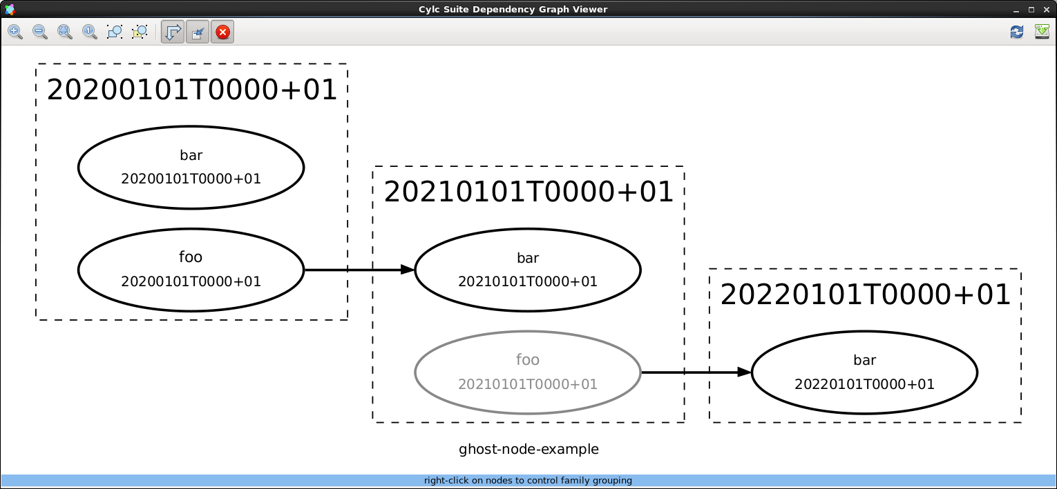
Fig. 29 Screenshot of cylc graph showing one task as a “ghost node”.
9.4. Runtime - Task Configuration
The [runtime] section of a suite configuration configures what
to execute (and where and how to execute it) when each task is ready to
run, in a multiple inheritance hierarchy of namespaces culminating in
individual tasks. This allows all common configuration detail to be
factored out and defined in one place.
Any namespace can configure any or all of the items defined in Suite.rc Reference.
Namespaces that do not explicitly inherit from others automatically inherit from the root namespace (below).
Nested namespaces define task families that can be used in the graph as convenient shorthand for triggering all member tasks at once, or for triggering other tasks off all members at once - see Family Triggers. Nested namespaces can be progressively expanded and collapsed in the dependency graph viewer, and in the gcylc graph and text views. Only the first parent of each namespace (as for single-inheritance) is used for suite visualization purposes.
9.4.1. Task and Namespace Names
There are restrictions on names that can be used for tasks and namespaces to ensure all tasks are processed and implemented correctly. Valid names must:
- begin with (or consist only of, as single-character task names are
allowed) either:
- an alphanumeric character, i.e. a letter in either upper or lower case
(
a-zorA-Z), or a digit (0-9); - an underscore (
_).
- an alphanumeric character, i.e. a letter in either upper or lower case
(
- otherwise contain only characters from the following options:
- alphanumeric characters or underscores (as above);
- any of these additional character symbols:
- hyphens (
-); - plus characters (
+); - percent signs (
%); - “at” signs (
@).
- hyphens (
- not be so long, typically over
255characters, as to raise errors from exceeding maximum filename length on the operating system for generated outputs e.g. directories named (in part) after the task they concern.
Warning
Task and namespace names may not contain colons (:), which would
preclude use of directory paths involving the registration name in
$PATH variables). They also may not contain the dot (.) character,
as it will be interpreted as the delimiter separating the task name from
an appended cycle point (see Task Identifiers).
Invalid names for tasks or namespaces will be raised as errors
by cylc validate.
Note
Task names need not be hardwired into task implementations because task and suite identity can be extracted portably from the task execution environment supplied by the suite server program (Task Execution Environment) - then to rename a task you can just change its name in the suite configuration.
9.4.2. Root - Runtime Defaults
The root namespace, at the base of the inheritance hierarchy, provides default configuration for all tasks in the suite. Most root items are unset by default, but some have default values sufficient to allow test suites to be defined by dependency graph alone. The script item, for example, defaults to code that prints a message then sleeps for between 1 and 15 seconds and exits. Default values are documented with each item in Suite.rc Reference. You can override the defaults or provide your own defaults by explicitly configuring the root namespace.
9.4.3. Defining Multiple Namespaces At Once
If a namespace section heading is a comma-separated list of names
then the subsequent configuration applies to each list member.
Particular tasks can be singled out at run time using the
$CYLC_TASK_NAME variable.
As an example, consider a suite containing an ensemble of closely related tasks that each invokes the same script but with a unique argument that identifies the calling task name:
[runtime]
    [[ENSEMBLE]]
        script = "run-model.sh $CYLC_TASK_NAME"
    [[m1, m2, m3]]
        inherit = ENSEMBLE
For large ensembles template processing can be used to automatically generate the member names and associated dependencies (see Jinja2 and EmPy).
9.4.4. Runtime Inheritance - Single
The following listing of the inherit.single.one example suite illustrates basic runtime inheritance with single parents.
# SUITE.RC
[meta]
    title = "User Guide [runtime] example."
[cylc]
    required run mode = simulation # (no task implementations)
[scheduling]
    initial cycle point = 20110101T06
    final cycle point = 20110102T00
    [[dependencies]]
        [[[T00]]]
            graph = """foo => OBS
                 OBS:succeed-all => bar"""
[runtime]
    [[root]] # base namespace for all tasks (defines suite-wide defaults)
        [[[job]]]
            batch system = at
        [[[environment]]]
            COLOR = red
    [[OBS]]  # family (inherited by land, ship); implicitly inherits root
        script = run-${CYLC_TASK_NAME}.sh
        [[[environment]]]
            RUNNING_DIR = $HOME/running/$CYLC_TASK_NAME
    [[land]] # a task (a leaf on the inheritance tree) in the OBS family
        inherit = OBS
        [[[meta]]]
            description = land obs processing
    [[ship]] # a task (a leaf on the inheritance tree) in the OBS family
        inherit = OBS
        [[[meta]]]
            description = ship obs processing
        [[[job]]]
            batch system = loadleveler
        [[[environment]]]
            RUNNING_DIR = $HOME/running/ship  # override OBS environment
            OUTPUT_DIR = $HOME/output/ship    # add to OBS environment
    [[foo]]
        # (just inherits from root)

    # The task [[bar]] is implicitly defined by its presence in the
    # graph; it is also a dummy task that just inherits from root.
9.4.5. Runtime Inheritance - Multiple
If a namespace inherits from multiple parents the linear order of precedence (which namespace overrides which) is determined by the so-called C3 algorithm used to find the linear method resolution order for class hierarchies in Python and several other object oriented programming languages. The result of this should be fairly obvious for typical use of multiple inheritance in cylc suites, but for detailed documentation of how the algorithm works refer to the official Python documentation.
The inherit.multi.one example suite, listed here, makes use of multiple inheritance:
[meta]
    title = "multiple inheritance example"

    description = """To see how multiple inheritance works:

 % cylc list -tb[m] SUITE # list namespaces
 % cylc graph -n SUITE # graph namespaces
 % cylc graph SUITE # dependencies, collapse on first-parent namespaces

  % cylc get-config --sparse --item [runtime]ops_s1 SUITE
  % cylc get-config --sparse --item [runtime]var_p2 foo"""

[scheduling]
    [[dependencies]]
        graph = "OPS:finish-all => VAR"

[runtime]
    [[root]]
    [[OPS]]
        script = echo "RUN: run-ops.sh"
    [[VAR]]
        script = echo "RUN: run-var.sh"
    [[SERIAL]]
        [[[directives]]]
            job_type = serial
    [[PARALLEL]]
        [[[directives]]]
            job_type = parallel
    [[ops_s1, ops_s2]]
        inherit = OPS, SERIAL

    [[ops_p1, ops_p2]]
        inherit = OPS, PARALLEL

    [[var_s1, var_s2]]
        inherit = VAR, SERIAL

    [[var_p1, var_p2]]
        inherit = VAR, PARALLEL

[visualization]
    # NOTE ON VISUALIZATION AND MULTIPLE INHERITANCE: overlapping
    # family groups can have overlapping attributes, so long as
    # non-conflictling attributes are used to style each group. Below,
    # for example, OPS tasks are filled green and SERIAL tasks are
    # outlined blue, so that ops_s1 and ops_s2 are green with a blue
    # outline. But if the SERIAL tasks are explicitly styled as "not
    # filled" (by setting "style=") this will override the fill setting
    # in the (previously defined and therefore lower precedence) OPS
    # group, making ops_s1 and ops_s2 unfilled with a blue outline.
    # Alternatively you can just create a manual node group for ops_s1
    # and ops_s2 and style them separately.
    [[node groups]]
        #(see comment above:)
        #serial_ops = ops_s1, ops_s2
    [[node attributes]]
        OPS = "style=filled", "fillcolor=green"
        SERIAL = "color=blue" #(see comment above:), "style="
        #(see comment above:)
        #serial_ops = "color=blue", "style=filled", "fillcolor=green"
cylc get-suite-config provides an easy way to check the result of
inheritance in a suite. You can extract specific items, e.g.:
$ cylc get-suite-config --item '[runtime][var_p2]script' \
    inherit.multi.one
echo ``RUN: run-var.sh''
or use the --sparse option to print entire namespaces
without obscuring the result with the dense runtime structure obtained
from the root namespace:
$ cylc get-suite-config --sparse --item '[runtime]ops_s1' inherit.multi.one
script = echo ``RUN: run-ops.sh''
inherit = ['OPS', 'SERIAL']
[directives]
   job_type = serial
9.4.5.1. Suite Visualization And Multiple Inheritance
The first parent inherited by a namespace is also used as the collapsible family group when visualizing the suite. If this is not what you want, you can demote the first parent for visualization purposes, without affecting the order of inheritance of runtime properties:
[runtime]
    [[BAR]]
        # ...
    [[foo]]
        # inherit properties from BAR, but stay under root for visualization:
        inherit = None, BAR
9.4.6. How Runtime Inheritance Works
The linear precedence order of ancestors is computed for each namespace using the C3 algorithm. Then any runtime items that are explicitly configured in the suite configuration are “inherited” up the linearized hierarchy for each task, starting at the root namespace: if a particular item is defined at multiple levels in the hierarchy, the level nearest the final task namespace takes precedence. Finally, root namespace defaults are applied for every item that has not been configured in the inheritance process (this is more efficient than carrying the full dense namespace structure through from root from the beginning).
9.4.7. Task Execution Environment
The task execution environment contains suite and task identity variables
provided by the suite server program, and user-defined environment variables.
The environment is explicitly exported (by the task job script) prior to
executing the task script (see Task Job Submission and Management).
Suite and task identity are exported first, so that user-defined variables can refer to them. Order of definition is preserved throughout so that variable assignment expressions can safely refer to previously defined variables.
Additionally, access to cylc itself is configured prior to the user-defined environment, so that variable assignment expressions can make use of cylc utility commands:
[runtime]
    [[foo]]
        [[[environment]]]
            REFERENCE_TIME = $( cylc util cycletime --offset-hours=6 )
9.4.7.1. User Environment Variables
A task’s user-defined environment results from its inherited
[[[environment]]] sections:
[runtime]
    [[root]]
        [[[environment]]]
            COLOR = red
            SHAPE = circle
    [[foo]]
        [[[environment]]]
            COLOR = blue  # root override
            TEXTURE = rough # new variable
This results in a task foo with SHAPE=circle, COLOR=blue,
and TEXTURE=rough in its environment.
9.4.7.2. Overriding Environment Variables
When you override inherited namespace items the original parent item definition is replaced by the new definition. This applies to all items including those in the environment sub-sections which, strictly speaking, are not “environment variables” until they are written, post inheritance processing, to the task job script that executes the associated task. Consequently, if you override an environment variable you cannot also access the original parent value:
[runtime]
    [[FOO]]
        [[[environment]]]
            COLOR = red
    [[bar]]
        inherit = FOO
        [[[environment]]]
            tmp = $COLOR        # !! ERROR: $COLOR is undefined here
            COLOR = dark-$tmp   # !! as this overrides COLOR in FOO.
The compressed variant of this, COLOR = dark-$COLOR, is
also in error for the same reason. To achieve the desired result you
must use a different name for the parent variable:
[runtime]
    [[FOO]]
        [[[environment]]]
            FOO_COLOR = red
    [[bar]]
        inherit = FOO
        [[[environment]]]
            COLOR = dark-$FOO_COLOR  # OK
9.4.7.3. Task Job Script Variables
These are variables that can be referenced (but should not be modified) in a task job script.
The task job script may export the following environment variables:
CYLC_DEBUG                      # Debug mode, true or not defined
CYLC_DIR                        # Location of cylc installation used
CYLC_VERSION                    # Version of cylc installation used

CYLC_CYCLING_MODE               # Cycling mode, e.g. gregorian
CYLC_SUITE_FINAL_CYCLE_POINT    # Final cycle point
CYLC_SUITE_INITIAL_CYCLE_POINT  # Initial cycle point
CYLC_SUITE_NAME                 # Suite name
CYLC_UTC                        # UTC mode, True or False
CYLC_VERBOSE                    # Verbose mode, True or False
TZ                              # Set to "UTC" in UTC mode or not defined

CYLC_SUITE_RUN_DIR              # Location of the suite run directory in
                                # job host, e.g. ~/cylc-run/foo
CYLC_SUITE_DEF_PATH             # Location of the suite configuration directory in
                                # job host, e.g. ~/cylc-run/foo
CYLC_SUITE_HOST                 # Host running the suite process
CYLC_SUITE_OWNER                # User ID running the suite process
CYLC_SUITE_DEF_PATH_ON_SUITE_HOST
                                # Location of the suite configuration directory in
                                # suite host, e.g. ~/cylc-run/foo
CYLC_SUITE_SHARE_DIR            # Suite (or task!) shared directory (see below)
CYLC_SUITE_UUID                 # Suite UUID string
CYLC_SUITE_WORK_DIR             # Suite work directory (see below)

CYLC_TASK_JOB                   # Task job identifier expressed as
                                # CYCLE-POINT/TASK-NAME/SUBMIT-NUM
                                # e.g. 20110511T1800Z/t1/01
CYLC_TASK_CYCLE_POINT           # Cycle point, e.g. 20110511T1800Z
CYLC_TASK_NAME                  # Job's task name, e.g. t1
CYLC_TASK_SUBMIT_NUMBER         # Job's submit number, e.g. 1,
                                # increments with every submit
CYLC_TASK_TRY_NUMBER            # Number of execution tries, e.g. 1
                                # increments with automatic retry-on-fail
CYLC_TASK_ID                    # Task instance identifier expressed as
                                # TASK-NAME.CYCLE-POINT
                                # e.g. t1.20110511T1800Z
CYLC_TASK_LOG_DIR               # Location of the job log directory
                                # e.g. ~/cylc-run/foo/log/job/20110511T1800Z/t1/01/
CYLC_TASK_LOG_ROOT              # The task job file path
                                # e.g. ~/cylc-run/foo/log/job/20110511T1800Z/t1/01/job
CYLC_TASK_WORK_DIR              # Location of task work directory (see below)
                                # e.g. ~/cylc-run/foo/work/20110511T1800Z/t1
CYLC_TASK_NAMESPACE_HIERARCHY   # Linearised family namespace of the task,
                                # e.g. root postproc t1
CYLC_TASK_DEPENDENCIES          # List of met dependencies that triggered the task
                                # e.g. foo.1 bar.1

CYLC_TASK_COMMS_METHOD          # Set to "ssh" if communication method is "ssh"
CYLC_TASK_SSH_LOGIN_SHELL       # With "ssh" communication, if set to "True",
                                # use login shell on suite host
There are also some global shell variables that may be defined in the task job script (but not exported to the environment). These include:
CYLC_FAIL_SIGNALS               # List of signals trapped by the error trap
CYLC_VACATION_SIGNALS           # List of signals trapped by the vacation trap
CYLC_SUITE_WORK_DIR_ROOT        # Root directory above the suite work directory
                                # in the job host
CYLC_TASK_MESSAGE_STARTED_PID   # PID of "cylc message" job started" command
CYLC_TASK_WORK_DIR_BASE         # Alternate task work directory,
                                # relative to the suite work directory
9.4.7.5. Task Work Directories
Task job scripts are executed from within work directories created
automatically under the suite run directory. A task can get its own work
directory from $CYLC_TASK_WORK_DIR (or simply $PWD if
it does not cd elsewhere at runtime). By default the location
contains task name and cycle point, to provide a unique workspace for every
instance of every task. This can be overridden in the suite configuration,
however, to get several tasks to share the same work directory
(see [runtime] -> [[__NAME__]] -> work sub-directory).
The top level work and share directory (above) location can be changed (e.g. to a large data area) by a global config setting (see [hosts] -> [[HOST]] -> work directory).
9.4.7.6. Environment Variable Evaluation
Variables in the task execution environment are not evaluated in the
shell in which the suite is running prior to submitting the task. They
are written in unevaluated form to the job script that is submitted by
cylc to run the task (Task Job Scripts) and are therefore
evaluated when the task begins executing under the task owner account
on the task host. Thus $HOME, for instance, evaluates at
run time to the home directory of task owner on the task host.
9.4.8. How Tasks Get Access To The Suite Directory
Tasks can use $CYLC_SUITE_DEF_PATH to access suite files on
the task host, and the suite bin directory is automatically added
$PATH. If a remote suite configuration directory is not
specified the local (suite host) path will be assumed with the local
home directory, if present, swapped for literal $HOME for
evaluation on the task host.
9.4.9. Remote Task Hosting
If a task declares an owner other than the suite owner and/or
a host other than the suite host, cylc will use non-interactive ssh to
execute the task on the owner@host account by the configured
batch system:
[runtime]
    [[foo]]
        [[[remote]]]
            host = orca.niwa.co.nz
            owner = bob
        [[[job]]]
            batch system = pbs
For this to work:
- non-interactive ssh is required from the suite host to the remote task accounts.
- cylc must be installed on task hosts.
- Optional software dependencies such as graphviz and Jinja2 are not needed on task hosts.
- If polling task communication is used, there is no other requirement.
- If SSH task communication is configured, non-interactive ssh is required from the task host to the suite host.
- If (default) task communication is configured, the task host should have access to the port on the suite host.
- the suite configuration directory, or some fraction of its content, can be installed on the task host, if needed.
To learn how to give remote tasks access to cylc, see Task Job Access To Cylc.
Tasks running on the suite host under another user account are treated as remote tasks.
Remote hosting, like all namespace settings, can be declared globally in the root namespace, or per family, or for individual tasks.
9.4.9.1. Dynamic Host Selection
Instead of hardwiring host names into the suite configuration you can specify a shell command that prints a hostname, or an environment variable that holds a hostname, as the value of the host config item. See [runtime] -> [[__NAME__]] -> [[[remote]]] -> host.
9.4.9.2. Remote Task Log Directories
Task stdout and stderr streams are written to log files in a suite-specific sub-directory of the suite run directory, as explained in Task stdout And stderr Logs. For remote tasks the same directory is used, but on the task host. Remote task log directories, like local ones, are created on the fly, if necessary, during job submission.
9.5. Visualization
The visualization section of a suite configuration is used to configure suite graphing, principally graph node (task) and edge (dependency arrow) style attributes. Tasks can be grouped for the purpose of applying common style attributes. See Suite.rc Reference for details.
9.5.1. Collapsible Families In Suite Graphs
[visualization]
    collapsed families = family1, family2
Nested families from the runtime inheritance hierarchy can be expanded
and collapsed in suite graphs and the gcylc graph view. All families
are displayed in the collapsed state at first, unless
[visualization]collapsed families is used to single out
specific families for initial collapsing.
In the gcylc graph view, nodes outside of the main graph (such as the members of collapsed families) are plotted as rectangular nodes to the right if they are doing anything interesting (submitted, running, failed).
Fig. 30 illustrates successive expansion of nested task families in the namespaces example suite.
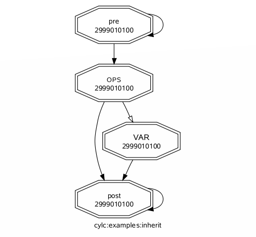
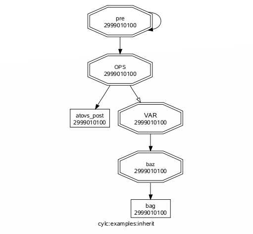
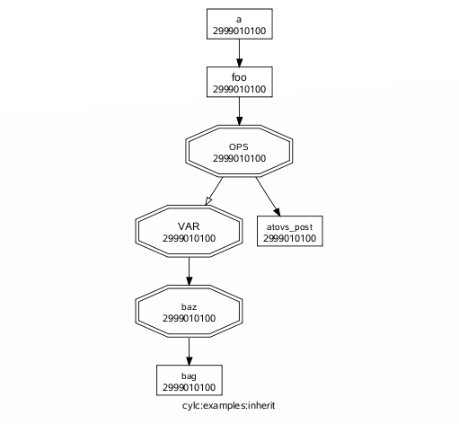
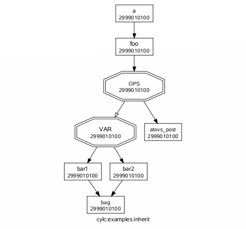
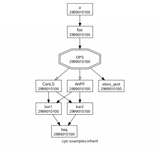
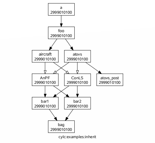
Fig. 30 Graphs of the namespaces example suite showing various states of expansion of the nested namespace family hierarchy, from all families collapsed (top left) through to all expanded (bottom right). This can also be done by right-clicking on tasks in the gcylc graph view.
9.6. Parameterized Tasks
Cylc can automatically generate tasks and dependencies by expanding parameterized task names over lists of parameter values. Uses for this include:
- generating an ensemble of similar model runs
- generating chains of tasks to process similar datasets
- replicating an entire workflow, or part thereof, over several runs
- splitting a long model run into smaller steps or
chunks(parameterized cycling)
Note
This can be done with Jinja2 loops too (Jinja2) but parameterization is much cleaner (nested loops can seriously reduce the clarity of a suite configuration).*
9.6.1. Parameter Expansion
Parameter values can be lists of strings, or lists of integers and integer ranges (with inclusive bounds). Numeric values in a list of strings are considered strings. It is not possible to mix strings with integer ranges.
For example:
[cylc]
    [[parameters]]
        # parameters: "ship", "buoy", "plane"
        # default task suffixes: _ship, _buoy, _plane
        obs = ship, buoy, plane

        # parameters: 1, 2, 3, 4, 5
        # default task suffixes: _run1, _run2, _run3, _run4, _run5
        run = 1..5

        # parameters: 1, 3, 5, 7, 9
        # default task suffixes: _idx1, _idx3, _idx5, _idx7, _idx9
        idx = 1..9..2

        # parameters: -11, -1, 9
        # default task suffixes: _idx-11, _idx-01, _idx+09
        idx = -11..9..10

        # parameters: 1, 3, 5, 10, 11, 12, 13
        # default task suffixes: _i01, _i03, _i05, _i10, _i11, _i12, _i13
        i = 1..5..2, 10, 11..13

        # parameters: "0", "1", "e", "pi", "i"
        # default task suffixes: _0, _1, _e, _pi, _i
        item = 0, 1, e, pi, i

        # ERROR: mix strings with int range
        p = one, two, 3..5
Then angle brackets denote use of these parameters throughout the suite configuration. For the values above, this parameterized name:
model<run> # for run = 1..5
expands to these concrete task names:
model_run1, model_run2, model_run3, model_run4, model_run5
and this parameterized name:
proc<obs> # for obs = ship, buoy, plane
expands to these concrete task names:
proc_ship, proc_buoy, proc_plane
By default, to avoid any ambiguity, the parameter name appears in the expanded
task names for integer values, but not for string values. For example,
model_run1 for run = 1, but proc_ship for
obs = ship. However, the default expansion templates can be
overridden if need be:
[cylc]
    [[parameters]]
        obs = ship, buoy, plane
        run = 1..5
    [[parameter templates]]
        run = -R%(run)s  # Make foo<run> expand to foo-R1 etc.
(See [cylc] -> [[parameter templates]] for more on the string template syntax.)
Any number of parameters can be used at once. This parameterization:
model<run,obs> # for run = 1..2 and obs = ship, buoy, plane
expands to these tasks names:
model_run1_ship, model_run1_buoy, model_run1_plane,
model_run2_ship, model_run2_buoy, model_run2_plane
Here’s a simple but complete example suite:
[cylc]
    [[parameters]]
        run = 1..2
[scheduling]
    [[dependencies]]
        graph = "prep => model<run>"
[runtime]
    [[model<run>]]
        # ...
The result, post parameter expansion, is this:
[scheduling]
    [[dependencies]]
        graph = "prep => model_run1 & model_run2"
[runtime]
    [[model_run1]]
        # ...
    [[model_run2]]
        # ...
Here’s a more complex graph using two parameters ([runtime] omitted):
[cylc]
    [[parameters]]
        run = 1..2
        mem = cat, dog
[scheduling]
    [[dependencies]]
        graph = """prep => init<run> => model<run,mem> =>
                      post<run,mem> => wrap<run> => done"""
Fig. 31 shows the result as visualized by
cylc graph.
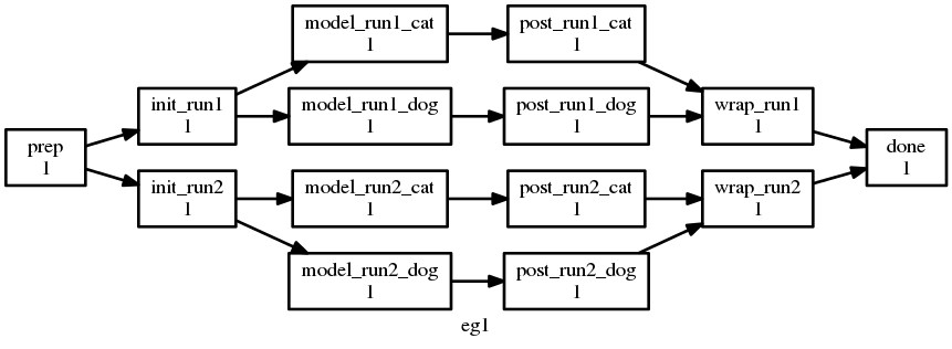
Fig. 31 Parameter expansion example.
9.6.1.1. Zero-Padded Integer Values
Integer parameter values are given a default template for generating task
suffixes that are zero-padded according to the longest size of their values.
For example, the default template for p = 9..10 would be
_p%(p)02d, so that foo<p> would become foo_p09, foo_p10.
If negative values are present in the parameter list, the
default template will include the sign.
For example, the default template for p = -1..1 would be
_p%(p)+02d, so that foo<p> would become
foo_p-1, foo_p+0, foo_p+1.
To get thicker padding and/or alternate suffixes, use a template. E.g.:
[cylc]
    [[parameters]]
        i = 1..9
        p = 3..14
    [[parameter templates]]
        i = _i%(i)02d  # suffixes = _i01, _i02, ..., _i09
        # A double-percent gives a literal percent character
        p = %%p%(p)03d  # suffixes = %p003, %p004, ..., %p013, %p014
9.6.1.2. Parameters as Full Task Names
Parameter values can be used as full task names, but the default template should be overridden to remove the initial underscore. For example:
[cylc]
    [[parameters]]
        i = 1..4
        obs = ship, buoy, plane
    [[parameter templates]]
        i = i%(i)d  # task name must begin with an alphabet
        obs = %(obs)s
[scheduling]
    [[dependencies]]
        graph = """
foo => <i>  # foo => i1 & i2 & i3 & i4
<obs> => bar  # ship & buoy & plane => bar
"""
9.6.2. Passing Parameter Values To Tasks
Parameter values are passed as environment variables to tasks generated by parameter expansion. For example, if we have:
[cylc]
    [[parameters]]
        obs = ship, buoy, plane
        run = 1..5
[scheduling]
    [[dependencies]]
        graph = model<run,obs>
Then task model_run2_ship would get the following standard
environment variables:
# In a job script of an instance of the "model_run2_ship" task:
export CYLC_TASK_PARAM_run="2"
export CYLC_TASK_PARAM_obs="ship"
These variables allow tasks to determine which member of a parameterized group they are, and so to vary their behaviour accordingly.
You can also define custom variables and string templates for parameter value substitution. For example, if we add this to the above configuration:
[runtime]
    [[model<run,obs>]]
        [[[environment]]]
            MYNAME = %(obs)sy-mc%(obs)sface
            MYFILE = /path/to/run%(run)03d/%(obs)s
Then task model_run2_ship would get the following custom
environment variables:
# In a job script of an instance of the "model_run2_ship" task:
export MYNAME MYFILE
MYNAME=shipy-mcshipface
MYFILE=/path/to/run002/ship
9.6.3. Selecting Specific Parameter Values
Specific parameter values can be singled out in the graph and under
[runtime] with the notation <p=5> (for example).
Here’s how to make a special task trigger off just the first of a
set of model runs:
[cylc]
    [[parameters]]
        run = 1..5
[scheduling]
    [[dependencies]]
        graph = """ model<run> => post_proc<run>  # general case
                    model<run=1> => check_first_run """  # special case
[runtime]
    [[model<run>]]
        # config for all "model" runs...
    [[model<run=1>]]
        # special config (if any) for the first model run...
    #...
9.6.4. Selecting Partial Parameter Ranges
The parameter notation does not currently support partial range selection such
as foo<p=5..10>, but you can achieve the same result by defining a
second parameter that covers the partial range and giving it the same expansion
template as the full-range parameter. For example:
[cylc]
    [[parameters]]
        run = 1..10  # 1, 2, ..., 10
        runx = 1..3  # 1, 2, 3
    [[parameter templates]]
        run = _R%(run)02d   # _R01, _R02, ..., _R10
        runx = _R%(runx)02d  # _R01, _R02, _R03
[scheduling]
    [[dependencies]]
        graph = """model<run> => post<run>
                   model<runx> => checkx<runx>"""
[runtime]
    [[model<run>]]
        # ...
    #...
9.6.5. Parameter Offsets In The Graph
A negative offset notation <NAME-1> is interpreted as the previous
value in the ordered list of parameter values, while a positive offset is
interpreted as the next value. For example, to split a model run into multiple
steps with each step depending on the previous one, either of these graphs:
graph = "model<run-1> => model<run>"  # for run = 1, 2, 3
graph = "model<run> => model<run+1>"  # for run = 1, 2, 3
expands to:
graph = """model_run1 => model_run2
           model_run2 => model_run3"""

# or equivalently:

graph = "model_run1 => model_run2 => model_run3"
And this graph:
graph = "proc<size-1> => proc<size>" # for size = small, big, huge
expands to:
graph = """proc_small => proc_big
           proc_big => proc_huge"""

# or equivalently:

graph = "proc_small => proc_big => proc_huge"
However, a quirk in the current system means that you should avoid mixing conditional logic in these statements. For example, the following will do the unexpected:
graph = foo<m-1> & baz => foo<m> # for m = cat, dog
currently expands to:
graph = foo_cat & baz => foo_dog

# when users may expect it to be:
#    graph = foo_cat => foo_dog
#    graph = baz => foo_cat & foo_dog
For the time being, writing out the logic explicitly will give you the correct graph.
graph = """foo<m-1> => foo<m>  # for m = cat, dog
           baz => foo<m>"""
9.6.6. Task Families And Parameterization
Task family members can be generated by parameter expansion:
[runtime]
    [[FAM]]
    [[member<r>]]
        inherit = FAM
# Result: family FAM contains member_r1, member_r2, etc.
Family names can be parameterized too, just like task names:
[runtime]
    [[RUN<r>]]
    [[model<r>]]
        inherit = RUN<r>
    [[post_proc<r>]]
        inherit = RUN<r>
# Result: family RUN_r1 contains model_r1 and post_proc_r1,
#         family RUN_r2 contains model_r2 and post_proc_r1, etc.
As described in Family Triggers family names can be used to trigger all members at once:
graph = "foo => FAMILY"
or to trigger off all members:
graph = "FAMILY:succeed-all => bar"
or to trigger off any members:
graph = "FAMILY:succeed-any => bar"
If the members of FAMILY were generated with parameters, you can
also trigger them all at once with parameter notation:
graph = "foo => member<m>"
Similarly, to trigger off all members:
graph = "member<m> => bar"
# (member<m>:fail etc., for other trigger types)
Family names are still needed in the graph, however, to succinctly express “succeed-any” triggering semantics, and all-to-all or any-to-all triggering:
graph = "FAM1:succeed-any => FAM2"
(Direct all-to-all and any-to-all family triggering is not recommended for efficiency reasons though - see Efficient Inter-Family Triggering).
For family member-to-member triggering use parameterized members.
For example, if family OBS_GET has members get<obs> and
family OBS_PROC has members proc<obs> then this graph:
graph = "get<obs> => proc<obs>" # for obs = ship, buoy, plane
expands to:
get_ship => proc_ship
get_buoy => proc_buoy
get_plane => proc_plane
9.6.7. Parameterized Cycling
Two ways of constructing cycling systems are described and contrasted in Workflows For Cycling Systems. For most purposes use of a proper cycling workflow is recommended, wherein cylc incrementally generates the date-time sequence and extends the workflow, potentially indefinitely, at run time. For smaller systems of finite duration, however, parameter expansion can be used to generate a sequence of pre-defined tasks as a proxy for cycling.
Here’s a cycling workflow of two-monthly model runs for one year, with previous-instance model dependence (e.g. for model restart files):
[scheduling]
    initial cycle point = 2020-01
    final cycle point = 2020-12
    [[dependencies]]
        [[[R1]]]  # Run once, at the initial point.
            graph = "prep => model"
        [[[P2M]]]  # Run at 2-month intervals between the initial and final points.
            graph = "model[-P2M] => model => post_proc & archive"
[runtime]
    [[model]]
        script = "run-model $CYLC_TASK_CYCLE_POINT"
And here’s how to do the same thing with parameterized tasks:
[cylc]
    [[parameters]]
        chunk = 1..6
[scheduling]
    [[dependencies]]
        graph = """prep => model<chunk=1>
                     model<chunk-1> => model<chunk> =>
                       post_proc<chunk> & archive<chunk>"""
[runtime]
    [[model<chunk>]]
        script = """
# Compute start date from chunk index and interval, then run the model.
INITIAL_POINT=2020-01
INTERVAL_MONTHS=2
OFFSET_MONTHS=(( (CYLC_TASK_PARAM_chunk - 1)*INTERVAL_MONTHS ))
OFFSET=P${OFFSET_MONTHS}M  # e.g. P4M for chunk=3
run-model $(cylc cyclepoint --offset=$OFFSET $INITIAL_POINT)"""
The two workflows are shown together in Fig. 32. They both achieve the same result, and both can include special tasks at the start, end, or anywhere in between. But as noted earlier the parameterized version has several disadvantages: it must be finite in extent and not too large; the date-time arithmetic has to be done by the user; and the full extent of the workflow will be visible at all times as the suite runs.
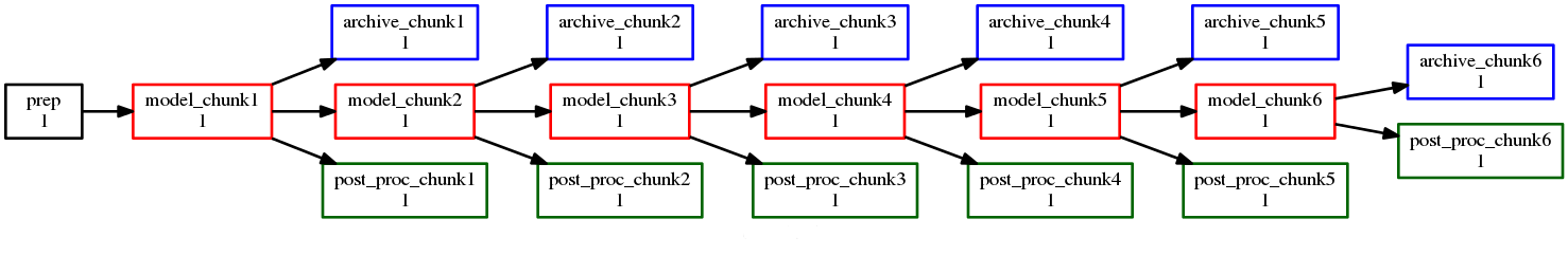
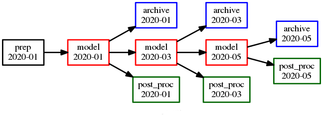
Fig. 32 Parameterized (top) and cycling (bottom) versions of the same workflow. The first three cycle points are shown in the cycling case. The parameterized case does not have “cycle points”.
Here’s a yearly-cycling suite with four parameterized chunks in each cycle point:
[cylc]
    [[parameters]]
        chunk = 1..4
[scheduling]
    initial cycle point = 2020-01
    [[dependencies]]
        [[[P1Y]]]
            graph = """model<chunk-1> => model<chunk>
                    model<chunk=4>[-P1Y] => model<chunk=1>"""
Note
The inter-cycle trigger connects the first chunk in each cycle point to the last chunk in the previous cycle point. Of course it would be simpler to just use 3-monthly cycling:
[scheduling]
    initial cycle point = 2020-01
    [[dependencies]]
        [[[P3M]]]
            graph = "model[-P3M] => model"
Here’s a possible valid use-case for mixed cycling: consider a portable date-time cycling workflow of model jobs that can each take too long to run on some supported platforms. This could be handled without changing the cycling structure of the suite by splitting the run (at each cycle point) into a variable number of shorter steps, using more steps on less powerful hosts.
9.6.7.1. Cycle Point And Parameter Offsets At Start-Up
In cycling workflows cylc ignores anything earlier than the suite initial cycle point. So this graph:
graph = "model[-P1D] => model"
simplifies at the initial cycle point to this:
graph = "model"
Similarly, parameter offsets are ignored if they extend beyond the start of the parameter value list. So this graph:
graph = "model<chunk-1> => model<chunk>"
simplifies for chunk=1 to this:
graph = "model_chunk1"
Note
The initial cut-off applies to every parameter list, but only to cycle point sequences that start at the suite initial cycle point. Therefore it may be somewhat easier to use parameterized cycling if you need multiple date-time sequences with different start points in the same suite. We plan to allow this sequence-start simplification for any date-time sequence in the future, not just at the suite initial point, but it needs to be optional because delayed-start cycling tasks sometimes need to trigger off earlier cycling tasks.
9.7. Jinja2
Note
This section needs to be revised - the Parameterized Task feature introduced in cylc-6.11.0 (see Parameterized Tasks) provides a cleaner way to auto-generate tasks without coding messy Jinja2 loops.
Cylc has built in support for the Jinja2 template processor in suite configurations. Jinja2 variables, mathematical expressions, loop control structures, conditional logic, etc., are automatically processed to generate the final suite configuration seen by cylc.
The need for Jinja2 processing must be declared with a hash-bang comment as the first line of the suite.rc file:
#!jinja2
# ...
Potential uses for this include automatic generation of repeated groups of similar tasks and dependencies, and inclusion or exclusion of entire suite sections according to the value of a single flag. Consider a large complicated operational suite and several related parallel test suites with slightly different task content and structure (the parallel suites, for instance, might take certain large input files from the operation or the archive rather than downloading them again) - these can now be maintained as a single master suite configuration that reconfigures itself according to the value of a flag variable indicating the intended use.
Template processing is the first thing done on parsing a suite configuration so Jinja2 expressions can appear anywhere in the file (inside strings and namespace headings, for example).
Jinja2 is well documented, so here we just provide an example suite that uses it. The meaning of the embedded Jinja2 code should be reasonably self-evident to anyone familiar with standard programming techniques.
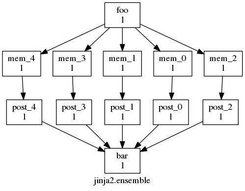
Fig. 33 The Jinja2 ensemble example suite graph.
The jinja2.ensemble example, graphed in
Fig. 33, shows an ensemble of similar tasks
generated using Jinja2:
#!jinja2
{% set N_MEMBERS = 5 %}
[scheduling]
    [[dependencies]]
        graph = """{# generate ensemble dependencies #}
            {% for I in range( 0, N_MEMBERS ) %}
               foo => mem_{{ I }} => post_{{ I }} => bar
            {% endfor %}"""
Here is the generated suite configuration, after Jinja2 processing:
#!jinja2
[scheduling]
    [[dependencies]]
        graph = """
          foo => mem_0 => post_0 => bar
          foo => mem_1 => post_1 => bar
          foo => mem_2 => post_2 => bar
          foo => mem_3 => post_3 => bar
          foo => mem_4 => post_4 => bar
                """
And finally, the jinja2.cities example uses variables,
includes or excludes special cleanup tasks according to the value of a
logical flag, and it automatically generates all dependencies and family
relationships for a group of tasks that is repeated for each city in the
suite. To add a new city and associated tasks and dependencies simply
add the city name to list at the top of the file. The suite is graphed,
with the New York City task family expanded, in
Fig. 34.
#!Jinja2
[meta]
    title = "Jinja2 city suite example."
    description = """
Illustrates use of variables and math expressions, and programmatic
generation of groups of related dependencies and runtime properties."""

{% set HOST = "SuperComputer" %}
{% set CITIES = 'NewYork', 'Philadelphia', 'Newark', 'Houston', 'SantaFe', 'Chicago' %}
{% set CITYJOBS = 'one', 'two', 'three', 'four' %}
{% set LIMIT_MINS = 20 %}

{% set CLEANUP = True %}

[scheduling]
    initial cycle point = 2011-08-08T12
    [[ dependencies ]]
{% if CLEANUP %}
        [[[T23]]]
            graph = "clean"
{% endif %}
        [[[T00,T12]]]
            graph = """
                    setup => get_lbc & get_ic # foo
{% for CITY in CITIES %} {# comment #}
                    get_lbc => {{ CITY }}_one
                    get_ic => {{ CITY }}_two
                    {{ CITY }}_one & {{ CITY }}_two => {{ CITY }}_three & {{ CITY }}_four
{% if CLEANUP %}
                    {{ CITY }}_three & {{ CITY }}_four => cleanup
{% endif %}
{% endfor %}
                    """
[runtime]
    [[on_{{ HOST }} ]]
        [[[remote]]]
            host = {{ HOST }}
            # (remote cylc directory is set in site/user config for this host)
        [[[directives]]]
            wall_clock_limit = "00:{{ LIMIT_MINS|int() + 2 }}:00,00:{{ LIMIT_MINS }}:00"

{% for CITY in CITIES %}
    [[ {{ CITY }} ]]
        inherit = on_{{ HOST }}
{% for JOB in CITYJOBS %}
    [[ {{ CITY }}_{{ JOB }} ]]
        inherit = {{ CITY }}
{% endfor %}
{% endfor %}

[visualization]
    initial cycle point = 2011-08-08T12
    final cycle point = 2011-08-08T23
    [[node groups]]
        cleaning = clean, cleanup
    [[node attributes]]
        cleaning = 'style=filled', 'fillcolor=yellow'
        NewYork = 'style=filled', 'fillcolor=lightblue'
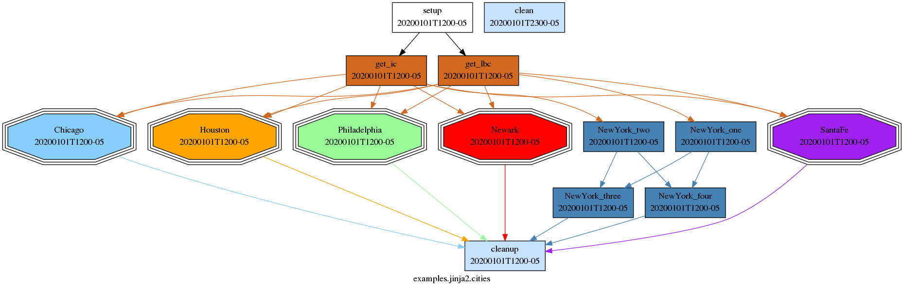
Fig. 34 The Jinja2 cities example suite graph, with the New York City task family expanded.
9.7.1. Accessing Environment Variables With Jinja2
This functionality is not provided by Jinja2 by default, but cylc automatically imports the user environment to template’s global namespace (see Custom Jinja2 Filters, Tests and Globals) in a dictionary structure called environ. A usage example:
#!Jinja2
#...
[runtime]
    [[root]]
        [[[environment]]]
            SUITE_OWNER_HOME_DIR_ON_SUITE_HOST = {{environ['HOME']}}
In addition, the following variables are exported to this environment prior to configuration parsing to provide suite context:
CYLC_DEBUG                      # Debug mode, true or not defined
CYLC_DIR                        # Location of cylc installation used
CYLC_VERBOSE                    # Verbose mode, True or False
CYLC_VERSION                    # Version of cylc installation used

CYLC_SUITE_NAME                 # Suite name

CYLC_SUITE_DEF_PATH             # Location of the suite configuration
                                # source path on suite host,
                                # e.g. ~/cylc-run/foo
CYLC_SUITE_LOG_DIR              # Suite log directory.
CYLC_SUITE_RUN_DIR              # Location of the suite run directory in
                                # suite host, e.g. ~/cylc-run/foo
CYLC_SUITE_SHARE_DIR            # Suite (or task post parsing!)
                                # shared directory.
CYLC_SUITE_WORK_DIR             # Suite work directory.
Note
The example above emphasizes that the environment - including the suite context variables - is read on the suite host when the suite configuration is parsed, not at task run time on job hosts.
9.7.2. Custom Jinja2 Filters, Tests and Globals
Jinja2 has three different namespaces used to separate “globals”, “filters” and “tests”. Globals are template-wide accessible variables and functions. Cylc extends this namespace with “environ” dictionary and “raise” and “assert” functions for raising exceptions (see Raising Exceptions).
Filters can be used to modify variable values and are applied using pipe
notation. For example, the built-in trim filter strips leading
and trailing white space from a string:
{% set MyString = "   dog   " %}
{{ MyString | trim() }}  # "dog"
Additionally, variable values can be tested using “is” keyword followed by
the name of the test, e.g. VARIABLE is defined.
See official Jinja2 documentation for available built-in globals, filters
and tests.
Cylc also supports custom Jinja2 globals, filters and tests. A custom global, filter or test is a single Python function in a source file with the same name as the function (plus “.py” extension) and stored in one of the following locations:
<cylc-dir>/lib/Jinja2[namespace]/[suite configuration directory]/Jinja2[namespace]/$HOME/.cylc/Jinja2[namespace]/
where [namespace]/ is one of Globals/, Filters/ or Tests/.
In the argument list of filter or test function, the first argument is the variable value to be “filtered” or “tested”, respectively, and subsequent arguments can be whatever else is needed. Currently there are three custom filters:
9.7.2.1. pad
The “pad” filter is for padding string values to some constant length with a fill character - useful for generating task names and related values in ensemble suites:
{% for i in range(0,100) %}  # 0, 1, ..., 99
    {% set j = i | pad(2,'0') %}
    [[A_{{j}}]]         # [[A_00]], [[A_01]], ..., [[A_99]]
{% endfor %}
9.7.2.2. strftime
The “strftime” filter can be used to format ISO8601 date-time strings using an strftime string.
{% set START_CYCLE = '10661004T08+01' %}
{{ START_CYCLE | strftime('%H') }}  # 00
Examples:
{{START_CYCLE | strftime('%Y')}}- 1066{{START_CYCLE | strftime('%m')}}- 10{{START_CYCLE | strftime('%d')}}- 14{{START_CYCLE | strftime('%H:%M:%S %z')}}- 08:00:00 +01
It is also possible to parse non-standard date-time strings by passing a strptime string as the second argument.
Examples:
{{'12,30,2000' | strftime('%m', '%m,%d,%Y')}}- 12{{'1066/10/14 08:00:00' | strftime('%Y%m%dT%H', '%Y/%m/%d %H:%M:%S')}}- 10661014T08
9.7.2.3. duration_as
The “duration_as” filter can be used to format ISO8601 duration strings as a floating-point number of several different units. Units for the conversion can be specified in a case-insensitive short or long form:
- Seconds - “s” or “seconds”
- Minutes - “m” or “minutes”
- Hours - “h” or “hours”
- Days - “d” or “days”
- Weeks - “w” or “weeks”
Within the suite, this becomes:
{% set CYCLE_INTERVAL = 'PT1D' %}
{{ CYCLE_INTERVAL | duration_as('h') }}  # 24.0
{% set CYCLE_SUBINTERVAL = 'PT30M' %}
{{ CYCLE_SUBINTERVAL | duration_as('hours') }}  # 0.5
{% set CYCLE_INTERVAL = 'PT1D' %}
{{ CYCLE_INTERVAL | duration_as('s') }}  # 86400.0
{% set CYCLE_SUBINTERVAL = 'PT30M' %}
{{ CYCLE_SUBINTERVAL | duration_as('seconds') }}  # 1800.0
While the filtered value is a floating-point number, it is often required to supply an integer to suite entities (e.g. environment variables) that require it. This is accomplished by chaining filters:
{{CYCLE_INTERVAL | duration_as('h') | int}}- 24{{CYCLE_SUBINTERVAL | duration_as('h') | int}}- 0{{CYCLE_INTERVAL | duration_as('s') | int}}- 86400{{CYCLE_SUBINTERVAL | duration_as('s') | int}}- 1800
9.7.3. Associative Arrays In Jinja2
Associative arrays (dicts in Python) can be very useful.
Here’s an example, from <cylc-dir>/etc/examples/jinja2/dict:
#!Jinja2
{% set obs_types = ['airs', 'iasi'] %}
{% set resource = { 'airs':'ncpus=9', 'iasi':'ncpus=20' } %}

[scheduling]
    [[dependencies]]
        graph = OBS
[runtime]
    [[OBS]]
        [[[job]]]
            batch system = pbs
    {% for i in obs_types %}
    [[ {{i}} ]]
        inherit = OBS
        [[[directives]]]
             -I = {{ resource[i] }}
     {% endfor %}
Here’s the result:
$ cylc get-suite-config -i [runtime][airs]directives SUITE
-I = ncpus=9
9.7.4. Jinja2 Default Values And Template Inputs
The values of Jinja2 variables can be passed in from the cylc command
line rather than hardwired in the suite configuration.
Here’s an example, from <cylc-dir>/etc/examples/jinja2/defaults:
#!Jinja2

[meta]

    title = "Jinja2 example: use of defaults and external input"

    description = """
The template variable FIRST_TASK must be given on the cylc command line
using --set or --set-file=FILE; two other variables, LAST_TASK and
N_MEMBERS can be set similarly, but if not they have default values."""

{% set LAST_TASK = LAST_TASK | default( 'baz' ) %}
{% set N_MEMBERS = N_MEMBERS | default( 3 ) | int %}

{# input of FIRST_TASK is required - no default #}

[scheduling]
    initial cycle point = 20100808T00
    final cycle point   = 20100816T00
    [[dependencies]]
        [[[0]]]
            graph = """{{ FIRST_TASK }} => ENS
                 ENS:succeed-all => {{ LAST_TASK }}"""
[runtime]
    [[ENS]]
{% for I in range( 0, N_MEMBERS ) %}
    [[ mem_{{ I }} ]]
        inherit = ENS
{% endfor %}
Here’s the result:
$ cylc list SUITE
Jinja2 Template Error
'FIRST_TASK' is undefined
cylc-list foo  failed:  1

$ cylc list --set FIRST_TASK=bob foo
bob
baz
mem_2
mem_1
mem_0

$ cylc list --set FIRST_TASK=bob --set LAST_TASK=alice foo
bob
alice
mem_2
mem_1
mem_0

$ cylc list --set FIRST_TASK=bob --set N_MEMBERS=10 foo
mem_9
mem_8
mem_7
mem_6
mem_5
mem_4
mem_3
mem_2
mem_1
mem_0
baz
bob
Note also that cylc view --set FIRST_TASK=bob --jinja2 SUITE
will show the suite with the Jinja2 variables as set.
Note
Suites started with template variables set on the command
line will restart with the same settings. However, you can set
them again on the cylc restart command line if they need to
be overridden.
9.7.5. Jinja2 Variable Scope
Jinja2 variable scoping rules may be surprising. Variables set inside a
for loop block, for instance, are not accessible outside of the block,
so the following will print # FOO is 0, not # FOO is 9:
{% set FOO = false %}
{% for item in items %}
    {% if item.check_something() %}
        {% set FOO = true %}
    {% endif %}
{% endfor %}
# FOO is {{FOO}}
Jinja2 documentation suggests using alternative constructs like the loop else
block or the special loop variable. More complex use cases can be
handled using namespace objects which allow propagating of changes
across scopes:
{% set ns = namespace(foo=false) %}
{% for item in items %}
    {% if item.check_something() %}
        {% set ns.foo = true %}
    {% endif %}
{% endfor %}
# FOO is {{ns.foo}}
For detail, see Jinja2 Template Designer Documentation > Assignments
9.7.6. Raising Exceptions
Cylc provides two functions for raising exceptions using Jinja2. These exceptions are raised when the suite.rc file is loaded and will prevent a suite from running.
Note
These functions must be contained within {{ Jinja2
blocks as opposed to {% blocks.
9.7.6.1. Raise
The “raise” function will result in an error containing the provided text.
{% if not VARIABLE is defined %}
    {{ raise('VARIABLE must be defined for this suite.') }}
{% endif %}
9.7.6.2. Assert
The “assert” function will raise an exception containing the text provided in the second argument providing that the first argument evaluates as False. The following example is equivalent to the “raise” example above.
{{ assert(VARIABLE is defined, 'VARIABLE must be defined for this suite.') }}
9.7.7. Importing additional Python modules
Jinja2 allows to gather variable and macro definitions in a separate template that can be imported into (and thus shared among) other templates.
{% import "suite-utils.rc" as utils %}
{% from "suite-utils.rc" import VARIABLE as ALIAS %}
{{ utils.VARIABLE is equalto(ALIAS)) }}
Cylc extends this functionality to allow import of arbitrary Python modules.
{% from "itertools" import product %}
[runtime]
{% for group, member in product(['a', 'b'], [0, 1, 2]) %}
    [[{{group}}_{{member}}]]
{% endfor %}
For better clarity and disambiguation Python modules can be prefixed with
__python__:
{% from "__python__.itertools" import product %}
9.8. EmPy
In addition to Jinja2, Cylc supports EmPy template processor in suite configurations. Similarly to Jinja2, EmPy provides variables, mathematical expressions, loop control structures, conditional logic, etc., that are expanded to generate the final suite configuration seen by Cylc. See the EmPy documentation for more details on its templating features and how to use them.
Note
EmPy is not bundled with Cylc and must be installed separately. It
should be available to Python through standard import em. Please also
note that there is another Python package called “em” that provides
a conflicting module of the same name. You can run
cylc check-software command to check your installation.
The need for EmPy processing must be declared with a hash-bang comment as the first line of the suite.rc file:
#!empy
# ...
An example suite empy.cities demonstrating its use is shown below.
It is a translation of jinja2.cities example from
Jinja2 and can be directly compared against it.
#!EmPy
[meta]
    title = "EmPy city suite example."
    description = """
Illustrates use of variables and math expressions, and programmatic
generation of groups of related dependencies and runtime properties.
"""

@{
HOST = "SuperComputer"
CITIES = 'NewYork', 'Philadelphia', 'Newark', 'Houston', 'SantaFe', 'Chicago'
CITYJOBS = 'one', 'two', 'three', 'four'
LIMIT_MINS = 20
CLEANUP = True
}

[scheduling]
    initial cycle point = 2011-08-08T12
    [[ dependencies ]]
@[ if CLEANUP ]
        [[[T23]]]
            graph = "clean"
@[ end if ]
        [[[T00,T12]]]
            graph = """
                setup => get_lbc & get_ic # foo
@[ for CITY in CITIES ]@# comment
                get_lbc => @(CITY)_one
                get_ic => @(CITY)_two
                @(CITY)_one & @(CITY)_two => @(CITY)_three & @(CITY)_four
    @[ if CLEANUP ]
                @(CITY)_three & @(CITY)_four => cleanup
    @[ end if ]
@[ end for ]
            """
[runtime]
    [[on_@HOST ]]
        [[[remote]]]
            host = @HOST
            # (remote cylc directory is set in site/user config for this host)
        [[[directives]]]
            wall_clock_limit = "00:@(LIMIT_MINS + 2):00,00:@(LIMIT_MINS):00"

@[ for CITY in CITIES ]
    [[ @(CITY) ]]
        inherit = on_@(HOST)
    @[ for JOB in CITYJOBS ]
    [[ @(CITY)_@(JOB) ]]
        inherit = @CITY
    @[ end for ]
@[ end for ]

@empy.include("./suite-visualization.rc")
For basic usage the difference between Jinja2 and EmPy amounts to a different markup syntax with little else to distinguish them. EmPy might be preferable, however, in cases where more complicated processing logic have to be implemented.
EmPy is a system for embedding Python expressions and statements in template text. It makes the full power of Python language and its ecosystem easily accessible from within the template. This might be desirable for several reasons:
- no need to learn different language and its idiosyncrasies just for writing template logic
- availability of lambda functions, list and dictionary comprehensions can make template code smaller and more readable compared to Jinja2
- natural and straightforward integration with Python package ecosystem
- no two-language barrier between writing template logic and processing extensions makes it easier to refactor and maintain the template code as its complexity grows - inline pieces of Python code can be gathered into subroutines and eventually into separate modules and packages in a seamless manner.
9.9. Omitting Tasks At Runtime
It is sometimes convenient to omit certain tasks from the suite at runtime without actually deleting their definitions from the suite.
Defining [runtime] properties for tasks that do not appear in the suite
graph results in verbose-mode validation warnings that the tasks are
disabled. They cannot be used because the suite graph is what defines
their dependencies and valid cycle points. Nevertheless, it is legal to
leave these orphaned runtime sections in the suite configuration because it
allows you to temporarily remove tasks from the suite by simply
commenting them out of the graph.
To omit a task from the suite at runtime but still leave it fully
defined and available for use (by insertion or cylc submit)
use one or both of [scheduling][[special task]] lists, include at
start-up or exclude at start-up (documented in [scheduling] -> [[special tasks]] -> include at start-up
and [scheduling] -> [[special tasks]] -> exclude at start-up). Then the graph still defines the
validity of the tasks and their dependencies, but they are not actually
loaded into the suite at start-up. Other tasks that depend on the
omitted ones, if any, will have to wait on their insertion at a later
time or otherwise be triggered manually.
Finally, with Jinja2 (Jinja2) you can radically alter
suite structure by including or excluding tasks from the [scheduling]
and [runtime] sections according to the value of a single logical flag
defined at the top of the suite.
9.10. Naked Dummy Tasks And Strict Validation
A naked dummy task appears in the suite graph but has no explicit runtime configuration section. Such tasks automatically inherit the default “dummy task” configuration from the root namespace. This is very useful because it allows functional suites to be mocked up quickly for test and demonstration purposes by simply defining the graph. It is somewhat dangerous, however, because there is no way to distinguish an intentional naked dummy task from one generated by typographic error: misspelling a task name in the graph results in a new naked dummy task replacing the intended task in the affected trigger expression; and misspelling a task name in a runtime section heading results in the intended task becoming a dummy task itself (by divorcing it from its intended runtime config section).
To avoid this problem any dummy task used in a real suite should not be
naked - i.e. it should have an explicit entry in under the runtime
section of the suite configuration, even if the section is empty. This
results in exactly the same dummy task behaviour, via implicit
inheritance from root, but it allows use of
cylc validate --strict
to catch errors in task names by failing the suite if any naked dummy
tasks are detected.
| [1] | An OR operator on the right doesn’t make much sense: if “B or C” triggers off A, what exactly should cylc do when A finishes? |
| [2] | In NWP forecast analysis suites parts of the observation processing and data assimilation subsystem will typically also depend on model background fields generated by the previous forecast. |